Autocorrelated Series – Application
Menghan Yuan
May 10, 2025
This script provides an example of autocorrelated residuals.
Dataset description
US Macroeconomics Data Set, Quarterly, 1950I to 2000IV, 204 Quarterly Observations
Source: Department of Commerce, BEA website and www.economagic.com
| Feild Name | Definition |
|---|---|
| year | Year |
| qtr | Quarter |
| realgdp | Real GDP ($bil) |
| realcons | Real consumption expenditures |
| realinvs | Real investment by private sector |
| realgovt | Real government expenditures |
| realdpi | Real disposable personal income |
| cpi_u | Consumer price index |
| M1 | Nominal money stock |
| tbilrate | Quarterly average of month end 90 day t bill rate |
| unemp | Unemployment rate |
| pop | Population, mil. interpolate of year end figures using constant growth rate per quarter |
| infl | Rate of inflation (First observation is missing) |
| realint | Ex post real interest rate = Tbilrate - Infl. (First observation is missing) |
# data preview
data <- read.table("https://raw.githubusercontent.com/my1396/course_dataset/refs/heads/main/TableF5-2.txt", header = TRUE)
data <- data %>%
    mutate(delta_infl = infl-lag(infl))
data %>%
    head() %>%
    knitr::kable(digits = 5) %>%
    kable_styling(bootstrap_options = c("striped", "hover"), full_width = FALSE, latex_options="scale_down") %>%
scroll_box(width = "100%")| Year | qtr | realgdp | realcons | realinvs | realgovt | realdpi | cpi_u | M1 | tbilrate | unemp | pop | infl | realint | delta_infl |
|---|---|---|---|---|---|---|---|---|---|---|---|---|---|---|
| 1950 | 1 | 1610.5 | 1058.9 | 198.1 | 361.0 | 1186.1 | 70.6 | 110.20 | 1.12 | 6.4 | 149.461 | 0.0000 | 0.0000 | |
| 1950 | 2 | 1658.8 | 1075.9 | 220.4 | 366.4 | 1178.1 | 71.4 | 111.75 | 1.17 | 5.6 | 150.260 | 4.5071 | -3.3404 | 4.5071 |
| 1950 | 3 | 1723.0 | 1131.0 | 239.7 | 359.6 | 1196.5 | 73.2 | 112.95 | 1.23 | 4.6 | 151.064 | 9.9590 | -8.7290 | 5.4519 |
| 1950 | 4 | 1753.9 | 1097.6 | 271.8 | 382.5 | 1210.0 | 74.9 | 113.93 | 1.35 | 4.2 | 151.871 | 9.1834 | -7.8301 | -0.7756 |
| 1951 | 1 | 1773.5 | 1122.8 | 242.9 | 421.9 | 1207.9 | 77.3 | 115.08 | 1.40 | 3.5 | 152.393 | 12.6160 | -11.2160 | 3.4326 |
| 1951 | 2 | 1803.7 | 1091.4 | 249.2 | 480.1 | 1225.8 | 77.6 | 116.19 | 1.53 | 3.1 | 152.917 | 1.5494 | -0.0161 | -11.0666 |
Empirical model
\[ \Delta I_t = \beta_1 + \beta_2 u_t + \varepsilon_t \] where
- \(I_t\) is the inflation rate; \(\Delta I_t = I_t - I_{t-1}\) is the first difference of the inflation rate;
- \(u_t\) is the unemployment rate;
- \(\varepsilon_t\) is the error term.
We remove the first two quarters due to missing value in the first observation and the change in the rate of inflation.
Regression result for OLS.
lm_phillips <- lm(delta_infl ~ unemp, data = data %>% tail(-2))
stargazer(lm_phillips,
type = "html",
title = "Phillips Curve Regression",
notes = "<span>*</span>: p<0.1; <span>**</span>: <strong>p<0.05</strong>; <span>***</span>: p<0.01 <br> Standard errors in parentheses.",
notes.append = F)| Dependent variable: | |
| delta_infl | |
| unemp | -0.090 |
| (0.126) | |
| Constant | 0.492 |
| (0.740) | |
| Observations | 202 |
| R2 | 0.003 |
| Adjusted R2 | -0.002 |
| Residual Std. Error | 2.822 (df = 200) |
| F Statistic | 0.513 (df = 1; 200) |
| Note: |
*: p<0.1; **: p<0.05; ***: p<0.01 Standard errors in parentheses. |
# variance-covariance matrix
vcov(lm_phillips)
## (Intercept) unemp
## (Intercept) 0.54830829 -0.08973175
## unemp -0.08973175 0.01582211Autocorrelated residuals
Plot the residuals.
plot(lm_phillips$residuals, type="l")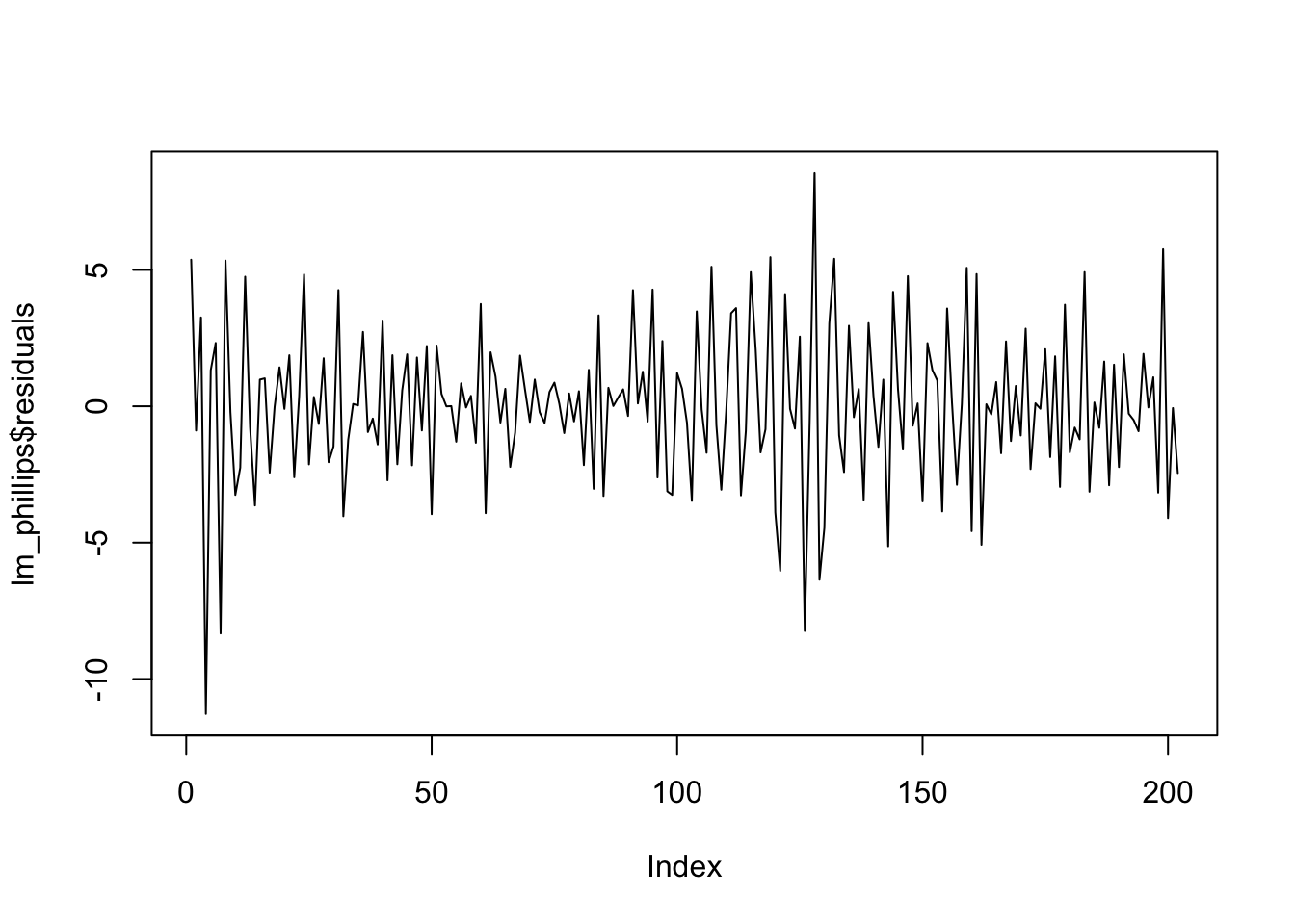
Fig. 1: Phillips Curve Deviations from Expected Inflation
Fig. 1 shows striking negative autocorrelation.
Now we test the serial correlation of the residuals. \[ \varepsilon_t = \phi\varepsilon_{t-1} + e_t \]
res <- tibble(
            res_t = lm_phillips$residuals,
            res_t1 = lag(lm_phillips$residuals))
lm_res <- lm(res_t ~ res_t1, data = res)
summary(lm_res)
##
## Call:
## lm(formula = res_t ~ res_t1, data = res)
##
## Residuals:
## Min 1Q Median 3Q Max
## -9.8694 -1.4800 0.0718 1.4990 8.3258
##
## Coefficients:
## Estimate Std. Error t value Pr(>|t|)
## (Intercept) -0.02155 0.17854 -0.121 0.904
## res_t1 -0.42630 0.06355 -6.708 2e-10 ***
## ---
## Signif. codes: 0 '***' 0.001 '**' 0.01 '*' 0.05 '.' 0.1 ' ' 1
##
## Residual standard error: 2.531 on 199 degrees of freedom
## (1 observation deleted due to missingness)
## Multiple R-squared: 0.1844, Adjusted R-squared: 0.1803
## F-statistic: 44.99 on 1 and 199 DF, p-value: 2.002e-10The regression of the least squares residuals on their past values gives a slope of -0.4263 with a highly significant \(t\) ratio of -6.7078. We thus conclude that the residuals in this models are highly negatively autocorrelated.
References:
- Ex. 12.3, Chap 12 Serial Correlation, Econometric Analysis, Greene 5th Edition, pp 251.