Equity Performance Evaluation
Menghan Yuan
March 27, 2024
Return Concepts
Simple returns
\(r_t\) measures the rate of return from \(t-1\) to \(t\). It is the percentage change in price given by:
\[ r_t = \frac{P_t-P_{t-1}}{P_{t-1}} = \frac{P_t}{P_{t-1}}-1 \]
One commonly used equality is
\[ P_t = P_{t-1} (1+r_t) \]
Continuously compounded returns
\(z_t\) measures the log return, also referred to as continuously compounded return. It is the first difference of the natural logarithm of prices.
\[ z_t = \ln P_t - \ln P_{t-1} = \ln \frac{P_t}{P_{t-1}} \]
The conversion between log return and simple return:
\[ \begin{aligned} \color{red}{z_t} &\color{red}{= \ln (1+r_t) }\\ r_t &= e^{z_t} -1 \end{aligned} \]
Q: Why is \(z_t\) continuously compounded return?
A: This is related to the constant \(e\), Euler number.
The discovery of the constant itself is credited to Jacob Bernoulli, who attempted to find the value of the following expression:
\[ e = \lim_{n\to\infty} \left( 1 + \frac{1}{n} \right)^n \]
If you put \(\$100\) in a bank with an annual interest rate of \(10\%\) and a yearly compounding period. What you get in a year can be expressed as follows:
\[ D_t = D_0 \left(1+\frac{R}{n}\right)^{nt} = 100\times \left(1+\frac{10\%}{1}\right)^{1\times1} = 110 \] Note that
\(\quad\) \(D_0\) is the initial deposit,
\(\quad\) \(D_t\) is the value of the deposit at time \(t\),
\(\quad\) \(R\) is the annual percentage rate (APR),
\(\quad\) \(n\) is the number of compounding periods in one year,
\(\quad\) \(t\) is the number of years from \(D_0\) to \(D_t\).
(For a bank deposit account, the quoted interest rate often refers to as “simple interest” which ignores compounding. For example, an interest rate of \(5\%\) payable every six months will be quoted as a simple interest of \(10\%\) per annum in the market.)
Q: What if we compound semi-annually?
A: That is when \(e\) equals 2.
\[ D_t = 100\times(1+\frac{10\%}{2})^{2\times1} = 110.25 \]
What if we compound monthly? \(\rightarrow\) \(n=12\)
\[ D_t = 100\times(1+\frac{10\%}{12})^{12\times1} = 110.47 \]
What if we compound daily? \(\rightarrow\) \(n=365\)
\[ D_t = 100\times(1+\frac{10\%}{365})^{365\times1} = 110.52 \]
\(\left(1+\frac{R}{n}\right)^{nt}\) can be rewritten as \(\left(1+\frac{1}{\frac{n}{R}}\right)^{\frac{n}{R} \cdot R \cdot t}\). We have
\[ \left(1+\frac{1}{\frac{n}{R}}\right)^{\frac{n}{R} \cdot R \cdot t} \to e^{Rt} \] as \(\frac{n}{R}\to \infty\).
Under continuous compounding,
\[ \color{red} {D_t = D_0\, e^{Rt}} . \]
R <- 0.1 # annual interest rate
t <- 1   # total time period

n <- 2 # compound frequency in one year
100 * (1+R/n)^{n*t}
## [1] 110.25n <- 12
100 * (1+R/n)^{n*t}## [1] 110.4713n <- 365
100 * (1+R/n)^{n*t}## [1] 110.5156100 * exp(R*t)## [1] 110.5171Note that
\(D_t\) under continuous compounding is always larger than those of under fixed compounding frequencies. The higher the frequency, the larger the end value \(D_t\) is. This is due to the earnings from “interest-on-interest”.
\(\left(1+\frac{R}{n}\right)^{n}-1\) is the effective interest rate. This is the interest rate you get as a proportion to the amount you put in and it depends on the frequency of compounding.
Continuously compounded interest rate is the effective interest rate when compounded continuously \((n\to\infty).\)
Proof. 1 Show \(\ln (1+x) \approx x\) as \(x\to 0\).
Let \(f(x)=\ln (1+x)\), its first-order Taylor expansion at \(x\) close to \(0\) is:
\[ \begin{aligned} f(x) \approx f(0) + f^\prime(0)(x-0) \end{aligned} \]
The first derivative of \(f(x)\) is
\[ f^\prime(x) = \frac{1}{1+x}. \]
Hence
\[ \begin{aligned} f(x) &\approx f(0) + f^\prime(0)(x-0) \\ &= \ln(1) + 1\cdot x \\ &= x. \end{aligned} \]
\(\square\)
From prices to returns.
f_name <- "data/Titlon_equity_price_2014-2023_daily.csv"
titlon_data <- read_csv(f_name)
## group by ISIN, calculate returns
titlon_group <- titlon_data %>% group_by(ISIN)
groups <- titlon_group %>% group_split()
group_key <- titlon_group %>%
    group_keys() %>%
    mutate(id = row_number())
group_key
## # A tibble: 501 × 2
## ISIN id
## <chr> <int>
## 1 AU000000CSS3 1
## 2 AU0000057408 2
## 3 BMG0451H1170 3
## 4 BMG0670A1099 4
## 5 BMG067231032 5
## 6 BMG0702P1086 6
## 7 BMG1466R1732 7
## 8 BMG1466R2078 8
## 9 BMG173841013 9
## 10 BMG1738J1247 10
## # ℹ 491 more rows# subset companies with more than 3 years' data
isin_vec <- titlon_group %>% tally() %>%
filter(n>(252*3)) %>%
pull(ISIN)
id_vec <- sapply(isin_vec, function(isin) which(group_key$ISIN==isin))
# data for one equity
i <- 4
groups[[id_vec[i]]]## # A tibble: 951 × 46
## Date `Internal code` SecurityId CompanyId Symbol ISIN Name
## <date> <dbl> <dbl> <dbl> <chr> <chr> <chr>
## 1 2020-02-19 2015535 1305295 12748 BWE BMG0702P1086 BW Energ…
## 2 2020-02-20 2015535 1305295 12748 BWE BMG0702P1086 BW Energ…
## 3 2020-02-21 2015535 1305295 12748 BWE BMG0702P1086 BW Energ…
## 4 2020-02-24 2015535 1305295 12748 BWE BMG0702P1086 BW Energ…
## 5 2020-02-25 2015535 1305295 12748 BWE BMG0702P1086 BW Energ…
## 6 2020-02-26 2015535 1305295 12748 BWE BMG0702P1086 BW Energ…
## 7 2020-02-27 2015535 1305295 12748 BWE BMG0702P1086 BW Energ…
## 8 2020-02-28 2015535 1305295 12748 BWE BMG0702P1086 BW Energ…
## 9 2020-03-02 2015535 1305295 12748 BWE BMG0702P1086 BW Energ…
## 10 2020-03-03 2015535 1305295 12748 BWE BMG0702P1086 BW Energ…
## BestBidPrice BestAskPrice Open High Low Close OfficialNumberOfTrades
## <dbl> <dbl> <dbl> <dbl> <dbl> <dbl> <dbl>
## 1 24.05 24.15 24.4 25 24 24.15 5661960
## 2 24.025 24.525 24.46 24.525 23.905 24.525 1669860
## 3 24.37 24.38 24.395 24.575 24.15 24.37 1088940
## 4 21.6 21.95 24.17 24.17 21 21.8 1493900
## 5 20.355 20.5 22.05 22.325 20.2 20.355 975605
## 6 19.648 19.742 20.2 20.335 18.702 19.742 1280330
## 7 17.35 17.6 19.468 19.468 16.728 17.35 1416090
## 8 17.028 17.3 17 19.29 16.22 17.028 1454460
## 9 17.2 17.294 18.1 18.5 17.2 17.294 1230160
## 10 19.2 19.55 17.75 19.9 16.976 19.55 1200440
## OfficialVolume Price AdjustedPrice Dividends LDividends CorpAdj DividendAdj
## <dbl> <dbl> <dbl> <dbl> <dbl> <dbl> <dbl>
## 1 138013000 24.15 24.15 0 NA 1 1
## 2 40391300 24.525 24.525 0 0 1 1
## 3 26567400 24.37 24.37 0 0 1 1
## 4 33336100 21.8 21.8 0 0 1 1
## 5 20524300 20.355 20.355 0 0 1 1
## 6 24942900 19.742 19.742 0 0 1 1
## 7 25110000 17.35 17.35 0 0 1 1
## 8 25091000 17.028 17.028 0 0 1 1
## 9 21635600 17.294 17.294 0 0 1 1
## 10 21580600 19.55 19.55 0 0 1 1
## Currency NumberOfShares Exchange NOKPerForex mktcap
## <chr> <dbl> <chr> <dbl> <dbl>
## 1 NOK 234304000 OB 1 5658450000
## 2 NOK 234304000 OB 1 5746310000
## 3 NOK 234304000 OB 1 5710000000
## 4 NOK 234304000 OB 1 5107830000
## 5 NOK 234304000 OB 1 4769260000
## 6 NOK 234304000 OB 1 4625640000
## 7 NOK 234304000 OB 1 4065180000
## 8 NOK 234304000 OB 1 3989730000
## 9 NOK 234304000 OB 1 4052060000
## 10 NOK 234304000 OB 1 4580650000
## OSEBXmktshare_prevmnth OSEBXAlpha_prevmnth OSEBXBeta_prevmnth SMB
## <dbl> <dbl> <dbl> <dbl>
## 1 NA NA NA -0.00499709
## 2 NA NA NA 0.000888762
## 3 NA NA NA 0.0158051
## 4 NA NA NA 0.0363824
## 5 NA NA NA 0.0141937
## 6 NA NA NA 0.00997761
## 7 NA NA NA 0.0313494
## 8 NA NA NA -0.0248113
## 9 NA NA NA 0.00952404
## 10 NA NA NA 0.000632531
## # ℹ 941 more rows
## # ℹ 16 more variables: HML <dbl>, LIQ <dbl>, MOM <dbl>, lnDeltaP <dbl>, lnDeltaOSEBX <dbl>, lnDeltaOBX <dbl>, NOWA_DayLnrate <dbl>, bills_3month_Lnrate <dbl>, Sector <chr>, IN_OSEBX <dbl>, Equity <dbl>, Debt <dbl>, Earnings <dbl>, debt_ratio <dbl>, PE <dbl>, ID <dbl>groups[[id_vec[i]]] %>% tail()## # A tibble: 6 × 46
## Date `Internal code` SecurityId CompanyId Symbol ISIN Name
## <date> <dbl> <dbl> <dbl> <chr> <chr> <chr>
## 1 2023-11-17 2015535 1305295 12748 BWE BMG0702P1086 BW ENERGY…
## 2 2023-11-20 2015535 1305295 12748 BWE BMG0702P1086 BW ENERGY…
## 3 2023-11-21 2015535 1305295 12748 BWE BMG0702P1086 BW ENERGY…
## 4 2023-11-22 2015535 1305295 12748 BWE BMG0702P1086 BW ENERGY…
## 5 2023-11-23 2015535 1305295 12748 BWE BMG0702P1086 BW ENERGY…
## 6 2023-11-24 2015535 1305295 12748 BWE BMG0702P1086 BW ENERGY…
## BestBidPrice BestAskPrice Open High Low Close OfficialNumberOfTrades
## <dbl> <dbl> <dbl> <dbl> <dbl> <dbl> <dbl>
## 1 26.2 25.8 26 26.05 25.05 25.85 659
## 2 25.7 25 25.7 26 25.2 25.55 455
## 3 25.8 24.05 25.55 25.7 24.5 24.5 546
## 4 25.6 23.8 25 25.05 24 24 559
## 5 25.6 23.85 24.4 24.75 24.05 24.1 452
## 6 25.7 23.8 24.05 24.35 23.9 24.25 435
## OfficialVolume Price AdjustedPrice Dividends LDividends CorpAdj DividendAdj
## <dbl> <dbl> <dbl> <dbl> <dbl> <dbl> <dbl>
## 1 593279 25.85 25.85 0 0 1 1
## 2 333063 25.55 25.55 0 0 1 1
## 3 454532 24.5 24.5 0 0 1 1
## 4 426403 24 24 0 0 1 1
## 5 343107 24.1 24.1 0 0 1 1
## 6 273388 24.25 24.25 0 0 1 1
## Currency NumberOfShares Exchange NOKPerForex mktcap OSEBXmktshare_prevmnth
## <chr> <dbl> <chr> <dbl> <dbl> <dbl>
## 1 NOK 257994000 XOSL 1 6669150000 NA
## 2 NOK 257994000 XOSL 1 6591750000 NA
## 3 NOK 257994000 XOSL 1 6320860000 NA
## 4 NOK 257994000 XOSL 1 6191860000 NA
## 5 NOK 257994000 XOSL 1 6217660000 NA
## 6 NOK 257994000 XOSL 1 6256360000 NA
## OSEBXAlpha_prevmnth OSEBXBeta_prevmnth SMB HML LIQ
## <dbl> <dbl> <dbl> <dbl> <dbl>
## 1 NA NA 0.000276874 0.00299032 0.00290608
## 2 NA NA -0.00214101 -0.00940512 0.00411524
## 3 NA NA 0.0047226 0.00645476 0.00897665
## 4 NA NA -0.00025938 0.0183181 0.00466264
## 5 NA NA 0.00145638 -0.00110734 -0.00304432
## 6 NA NA 0.0063141 0.00882244 -0.00237105
## # ℹ 14 more variables: MOM <dbl>, lnDeltaP <dbl>, lnDeltaOSEBX <dbl>, lnDeltaOBX <dbl>, NOWA_DayLnrate <dbl>, bills_3month_Lnrate <dbl>, Sector <chr>, IN_OSEBX <dbl>, Equity <dbl>, Debt <dbl>, Earnings <dbl>, debt_ratio <dbl>, PE <dbl>, ID <dbl>the_group <- groups[[id_vec[i]]]
the_group## # A tibble: 951 × 46
## Date `Internal code` SecurityId CompanyId Symbol ISIN Name
## <date> <dbl> <dbl> <dbl> <chr> <chr> <chr>
## 1 2020-02-19 2015535 1305295 12748 BWE BMG0702P1086 BW Energ…
## 2 2020-02-20 2015535 1305295 12748 BWE BMG0702P1086 BW Energ…
## 3 2020-02-21 2015535 1305295 12748 BWE BMG0702P1086 BW Energ…
## 4 2020-02-24 2015535 1305295 12748 BWE BMG0702P1086 BW Energ…
## 5 2020-02-25 2015535 1305295 12748 BWE BMG0702P1086 BW Energ…
## 6 2020-02-26 2015535 1305295 12748 BWE BMG0702P1086 BW Energ…
## 7 2020-02-27 2015535 1305295 12748 BWE BMG0702P1086 BW Energ…
## 8 2020-02-28 2015535 1305295 12748 BWE BMG0702P1086 BW Energ…
## 9 2020-03-02 2015535 1305295 12748 BWE BMG0702P1086 BW Energ…
## 10 2020-03-03 2015535 1305295 12748 BWE BMG0702P1086 BW Energ…
## BestBidPrice BestAskPrice Open High Low Close OfficialNumberOfTrades
## <dbl> <dbl> <dbl> <dbl> <dbl> <dbl> <dbl>
## 1 24.05 24.15 24.4 25 24 24.15 5661960
## 2 24.025 24.525 24.46 24.525 23.905 24.525 1669860
## 3 24.37 24.38 24.395 24.575 24.15 24.37 1088940
## 4 21.6 21.95 24.17 24.17 21 21.8 1493900
## 5 20.355 20.5 22.05 22.325 20.2 20.355 975605
## 6 19.648 19.742 20.2 20.335 18.702 19.742 1280330
## 7 17.35 17.6 19.468 19.468 16.728 17.35 1416090
## 8 17.028 17.3 17 19.29 16.22 17.028 1454460
## 9 17.2 17.294 18.1 18.5 17.2 17.294 1230160
## 10 19.2 19.55 17.75 19.9 16.976 19.55 1200440
## OfficialVolume Price AdjustedPrice Dividends LDividends CorpAdj DividendAdj
## <dbl> <dbl> <dbl> <dbl> <dbl> <dbl> <dbl>
## 1 138013000 24.15 24.15 0 NA 1 1
## 2 40391300 24.525 24.525 0 0 1 1
## 3 26567400 24.37 24.37 0 0 1 1
## 4 33336100 21.8 21.8 0 0 1 1
## 5 20524300 20.355 20.355 0 0 1 1
## 6 24942900 19.742 19.742 0 0 1 1
## 7 25110000 17.35 17.35 0 0 1 1
## 8 25091000 17.028 17.028 0 0 1 1
## 9 21635600 17.294 17.294 0 0 1 1
## 10 21580600 19.55 19.55 0 0 1 1
## Currency NumberOfShares Exchange NOKPerForex mktcap
## <chr> <dbl> <chr> <dbl> <dbl>
## 1 NOK 234304000 OB 1 5658450000
## 2 NOK 234304000 OB 1 5746310000
## 3 NOK 234304000 OB 1 5710000000
## 4 NOK 234304000 OB 1 5107830000
## 5 NOK 234304000 OB 1 4769260000
## 6 NOK 234304000 OB 1 4625640000
## 7 NOK 234304000 OB 1 4065180000
## 8 NOK 234304000 OB 1 3989730000
## 9 NOK 234304000 OB 1 4052060000
## 10 NOK 234304000 OB 1 4580650000
## OSEBXmktshare_prevmnth OSEBXAlpha_prevmnth OSEBXBeta_prevmnth SMB
## <dbl> <dbl> <dbl> <dbl>
## 1 NA NA NA -0.00499709
## 2 NA NA NA 0.000888762
## 3 NA NA NA 0.0158051
## 4 NA NA NA 0.0363824
## 5 NA NA NA 0.0141937
## 6 NA NA NA 0.00997761
## 7 NA NA NA 0.0313494
## 8 NA NA NA -0.0248113
## 9 NA NA NA 0.00952404
## 10 NA NA NA 0.000632531
## # ℹ 941 more rows
## # ℹ 16 more variables: HML <dbl>, LIQ <dbl>, MOM <dbl>, lnDeltaP <dbl>, lnDeltaOSEBX <dbl>, lnDeltaOBX <dbl>, NOWA_DayLnrate <dbl>, bills_3month_Lnrate <dbl>, Sector <chr>, IN_OSEBX <dbl>, Equity <dbl>, Debt <dbl>, Earnings <dbl>, debt_ratio <dbl>, PE <dbl>, ID <dbl>ticker <- the_group$Symbol[1]
ticker## [1] "BWE"the_group$Name[1]## [1] "BW Energy Limited"# convert to xts
library(quantmod)
the_group_xts <- xts(the_group[,c("AdjustedPrice")], order.by=the_group$Date)
# the_group_xts <- xts(the_group[,c("Price")], order.by=the_group$Date)
the_group_xts %>% str()## An xts object on 2020-02-19 / 2023-11-24 containing:
## Data: double [951, 1]
## Columns: AdjustedPrice
## Index: Date [951] (TZ: "UTC")the_group_xts## AdjustedPrice
## 2020-02-19 24.150
## 2020-02-20 24.525
## 2020-02-21 24.370
## 2020-02-24 21.800
## 2020-02-25 20.355
## 2020-02-26 19.742
## 2020-02-27 17.350
## 2020-02-28 17.028
## 2020-03-02 17.294
## 2020-03-03 19.550
## ...
## 2023-11-13 29.300
## 2023-11-14 28.850
## 2023-11-15 28.750
## 2023-11-16 26.100
## 2023-11-17 25.850
## 2023-11-20 25.550
## 2023-11-21 24.500
## 2023-11-22 24.000
## 2023-11-23 24.100
## 2023-11-24 24.250# from daily to monthly
prices_monthly <- the_group_xts %>% to.monthly(indexAt = "last", OHLC=FALSE)
prices_monthly %>% head(20)## AdjustedPrice
## 2020-02-28 17.028
## 2020-03-31 9.070
## 2020-04-30 12.740
## 2020-05-29 14.554
## 2020-06-30 17.168
## 2020-07-31 17.170
## 2020-08-31 20.500
## 2020-09-30 16.750
## 2020-10-30 14.800
## 2020-11-30 20.920
## 2020-12-30 27.600
## 2021-01-29 24.180
## 2021-02-26 25.160
## 2021-03-31 26.880
## 2021-04-30 27.750
## 2021-05-31 23.950
## 2021-06-30 26.200
## 2021-07-30 26.750
## 2021-08-31 27.950
## 2021-09-30 27.900prices_monthly %>% tail(20)## AdjustedPrice
## 2022-04-29 27.50
## 2022-05-31 28.84
## 2022-06-30 25.56
## 2022-07-29 27.42
## 2022-08-31 24.82
## 2022-09-30 21.62
## 2022-10-31 26.30
## 2022-11-30 27.06
## 2022-12-30 25.14
## 2023-01-31 27.90
## 2023-02-28 29.24
## 2023-03-31 26.92
## 2023-04-28 28.60
## 2023-05-31 27.25
## 2023-06-30 25.80
## 2023-07-31 30.00
## 2023-08-31 25.65
## 2023-09-29 27.35
## 2023-10-31 27.90
## 2023-11-24 24.25# price plot
plot(prices_monthly, main = sprintf("Monthly Price: %s", ticker))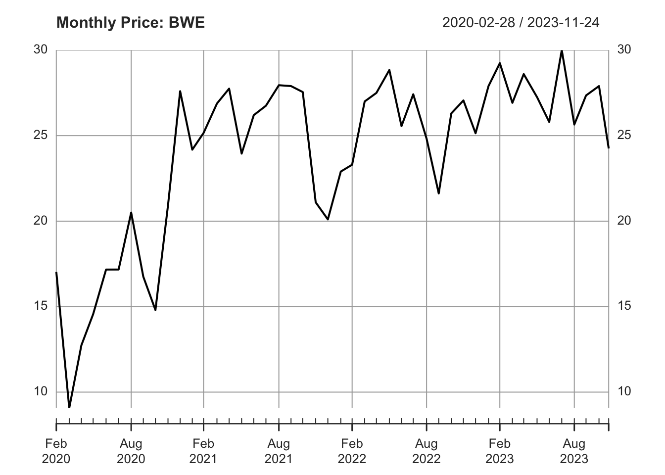
# calculate monthly return by hand
simple_ret <- (diff(prices_monthly)/lag(prices_monthly)) %>% setNames("simple_return") # simple return
log_ret <- diff(log(prices_monthly)) %>% setNames("log_return")   # log return, aka, continuously compounded return
merge(prices_monthly, simple_ret, log_ret)
## AdjustedPrice simple_return log_return
## 2020-02-28 17.028 NA NA
## 2020-03-31 9.070 -0.4673478976 -0.629886784
## 2020-04-30 12.740 0.4046306505 0.339774386
## 2020-05-29 14.554 0.1423861852 0.133119220
## 2020-06-30 17.168 0.1796069809 0.165181316
## 2020-07-31 17.170 0.0001164958 0.000116489
## 2020-08-31 20.500 0.1939429237 0.177261211
## 2020-09-30 16.750 -0.1829268293 -0.202026628
## 2020-10-30 14.800 -0.1164179104 -0.123771078
## 2020-11-30 20.920 0.4135135135 0.346078458
## 2020-12-30 27.600 0.3193116635 0.277110134
## 2021-01-29 24.180 -0.1239130435 -0.132289928
## 2021-02-26 25.160 0.0405293631 0.039729587
## 2021-03-31 26.880 0.0683624801 0.066127084
## 2021-04-30 27.750 0.0323660714 0.031853325
## 2021-05-31 23.950 -0.1369369369 -0.147267516
## 2021-06-30 26.200 0.0939457203 0.089791087
## 2021-07-30 26.750 0.0209923664 0.020775063
## 2021-08-31 27.950 0.0448598131 0.043882726
## 2021-09-30 27.900 -0.0017889088 -0.001790511
## 2021-10-29 27.550 -0.0125448029 -0.012624153
## 2021-11-30 21.100 -0.2341197822 -0.266729495
## 2021-12-30 20.100 -0.0473933649 -0.048553225
## 2022-01-31 22.900 0.1393034826 0.130417095
## 2022-02-28 23.300 0.0174672489 0.017316450
## 2022-03-31 27.000 0.1587982833 0.147383505
## 2022-04-29 27.500 0.0185185185 0.018349139
## 2022-05-31 28.840 0.0487272727 0.047577308
## 2022-06-30 25.560 -0.1137309293 -0.120734683
## 2022-07-29 27.420 0.0727699531 0.070244045
## 2022-08-31 24.820 -0.0948212983 -0.099622894
## 2022-09-30 21.620 -0.1289282836 -0.138030968
## 2022-10-31 26.300 0.2164662350 0.195950127
## 2022-11-30 27.060 0.0288973384 0.028487684
## 2022-12-30 25.140 -0.0709534368 -0.073596420
## 2023-01-31 27.900 0.1097852029 0.104166486
## 2023-02-28 29.240 0.0480286738 0.046910946
## 2023-03-31 26.920 -0.0793433653 -0.082668130
## 2023-04-28 28.600 0.0624071322 0.060537213
## 2023-05-31 27.250 -0.0472027972 -0.048353197
## 2023-06-30 25.800 -0.0532110092 -0.054679029
## 2023-07-31 30.000 0.1627906977 0.150822890
## 2023-08-31 25.650 -0.1450000000 -0.156653810
## 2023-09-29 27.350 0.0662768031 0.064172957
## 2023-10-31 27.900 0.0201096892 0.019910160
## 2023-11-24 24.250 -0.1308243728 -0.140210071# calculate monthly return using `PerformanceAnalytics::Return.calculate`
library(PerformanceAnalytics)
merge(Return.calculate(prices_monthly, method = "discrete"),
Return.calculate(prices_monthly, method = "log") ) %>%
fortify() %>%
setNames(c("Date", "Simple Ret", "Log Ret")) %>%
knitr::kable(digits = 5, escape=F, caption="Using `PerformanceAnalytics::Return.calculate`") %>%
kable_styling(bootstrap_options = c("striped", "hover"), full_width = F, latex_options="scale_down") %>%
scroll_box(height = "500px")| Date | Simple Ret | Log Ret |
|---|---|---|
| 2020-02-28 | ||
| 2020-03-31 | -0.46735 | -0.62989 |
| 2020-04-30 | 0.40463 | 0.33977 |
| 2020-05-29 | 0.14239 | 0.13312 |
| 2020-06-30 | 0.17961 | 0.16518 |
| 2020-07-31 | 0.00012 | 0.00012 |
| 2020-08-31 | 0.19394 | 0.17726 |
| 2020-09-30 | -0.18293 | -0.20203 |
| 2020-10-30 | -0.11642 | -0.12377 |
| 2020-11-30 | 0.41351 | 0.34608 |
| 2020-12-30 | 0.31931 | 0.27711 |
| 2021-01-29 | -0.12391 | -0.13229 |
| 2021-02-26 | 0.04053 | 0.03973 |
| 2021-03-31 | 0.06836 | 0.06613 |
| 2021-04-30 | 0.03237 | 0.03185 |
| 2021-05-31 | -0.13694 | -0.14727 |
| 2021-06-30 | 0.09395 | 0.08979 |
| 2021-07-30 | 0.02099 | 0.02078 |
| 2021-08-31 | 0.04486 | 0.04388 |
| 2021-09-30 | -0.00179 | -0.00179 |
| 2021-10-29 | -0.01254 | -0.01262 |
| 2021-11-30 | -0.23412 | -0.26673 |
| 2021-12-30 | -0.04739 | -0.04855 |
| 2022-01-31 | 0.13930 | 0.13042 |
| 2022-02-28 | 0.01747 | 0.01732 |
| 2022-03-31 | 0.15880 | 0.14738 |
| 2022-04-29 | 0.01852 | 0.01835 |
| 2022-05-31 | 0.04873 | 0.04758 |
| 2022-06-30 | -0.11373 | -0.12073 |
| 2022-07-29 | 0.07277 | 0.07024 |
| 2022-08-31 | -0.09482 | -0.09962 |
| 2022-09-30 | -0.12893 | -0.13803 |
| 2022-10-31 | 0.21647 | 0.19595 |
| 2022-11-30 | 0.02890 | 0.02849 |
| 2022-12-30 | -0.07095 | -0.07360 |
| 2023-01-31 | 0.10979 | 0.10417 |
| 2023-02-28 | 0.04803 | 0.04691 |
| 2023-03-31 | -0.07934 | -0.08267 |
| 2023-04-28 | 0.06241 | 0.06054 |
| 2023-05-31 | -0.04720 | -0.04835 |
| 2023-06-30 | -0.05321 | -0.05468 |
| 2023-07-31 | 0.16279 | 0.15082 |
| 2023-08-31 | -0.14500 | -0.15665 |
| 2023-09-29 | 0.06628 | 0.06417 |
| 2023-10-31 | 0.02011 | 0.01991 |
| 2023-11-24 | -0.13082 | -0.14021 |
Cumulative returns
For simple return, the cumulative return from time \(0\) to time \(T\) is given by:
\[ r_{0:T} = \Pi_{t=1}^T (1+r_t) -1. \]
For log return
\[ z_{0:T} = \sum_{t=1}^T z_t \]
Note that we have to back out the simple return from the log return
\[ r_{0:T} = \exp(z_{0:T}) -1 \]
return_monthly_simple <- Return.calculate(prices_monthly, method = "discrete")
return_monthly_simple[1,] <- 0
cumulative_returns_simple <- cumprod(1 + return_monthly_simple) - 1
# plot price, monthly ret, and cumu ret
par(mfrow=c(3,1))
plot(prices_monthly, main = sprintf("Monthly adjPrice: %s", ticker))
plot(return_monthly_simple,
     main = sprintf("Monthly Return: %s", ticker))
plot(cumulative_returns_simple,
     main = sprintf("Monthly Cumulative Return: %s", ticker))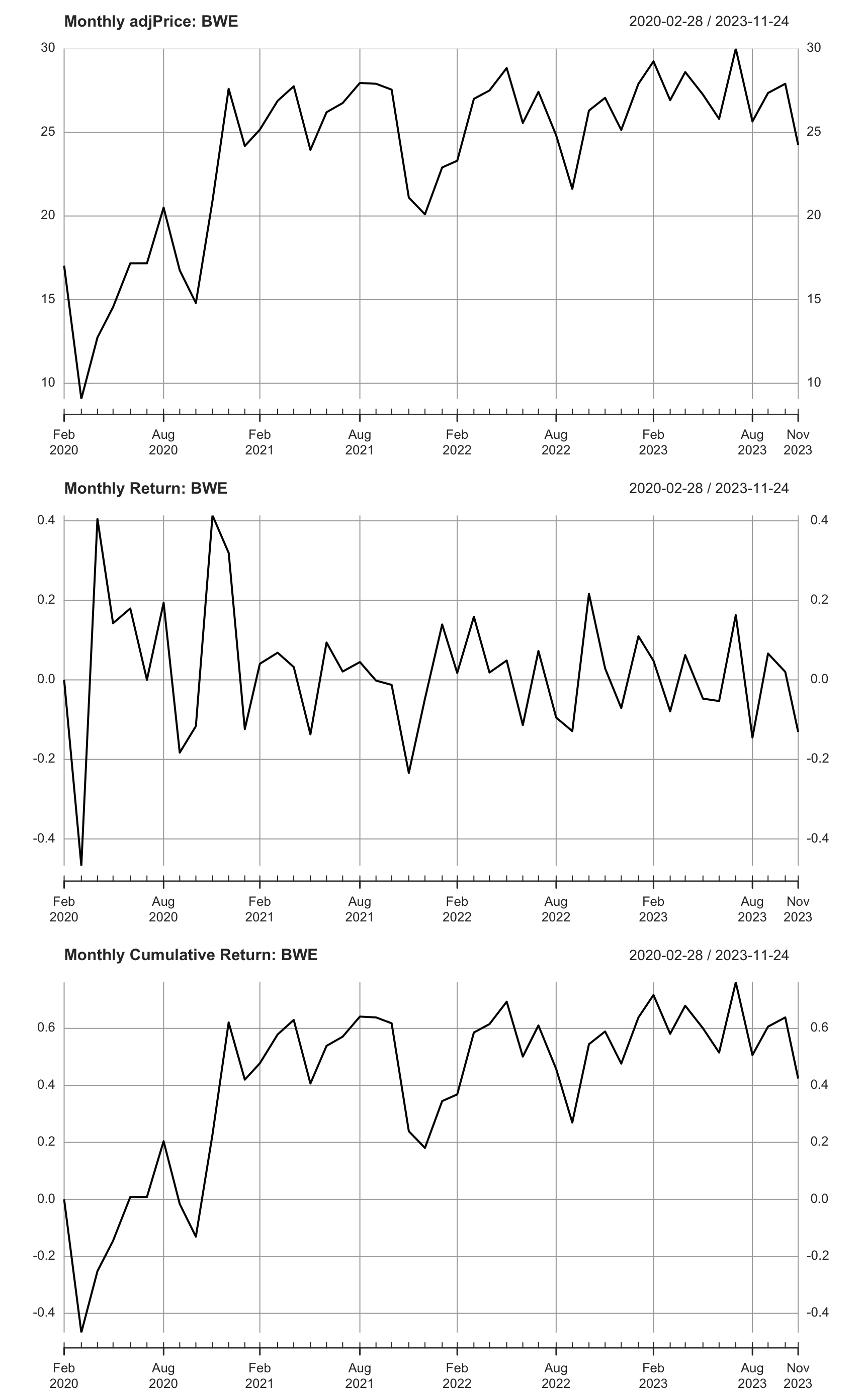
Fig. 1: Simple returns
return_monthly_log <- Return.calculate(prices_monthly, method = "log")
return_monthly_log[1,] <- 0
cumulative_returns_log <- exp(cumsum(return_monthly_log)) - 1 # back out the simple return
par(mfrow=c(3,1))
plot(prices_monthly, main = sprintf("Monthly adjPrice: %s", ticker))
plot(return_monthly_log,
     main = sprintf("Monthly Return: %s", ticker))
plot(cumulative_returns_log,
     main = sprintf("Monthly Cumulative Return: %s", ticker))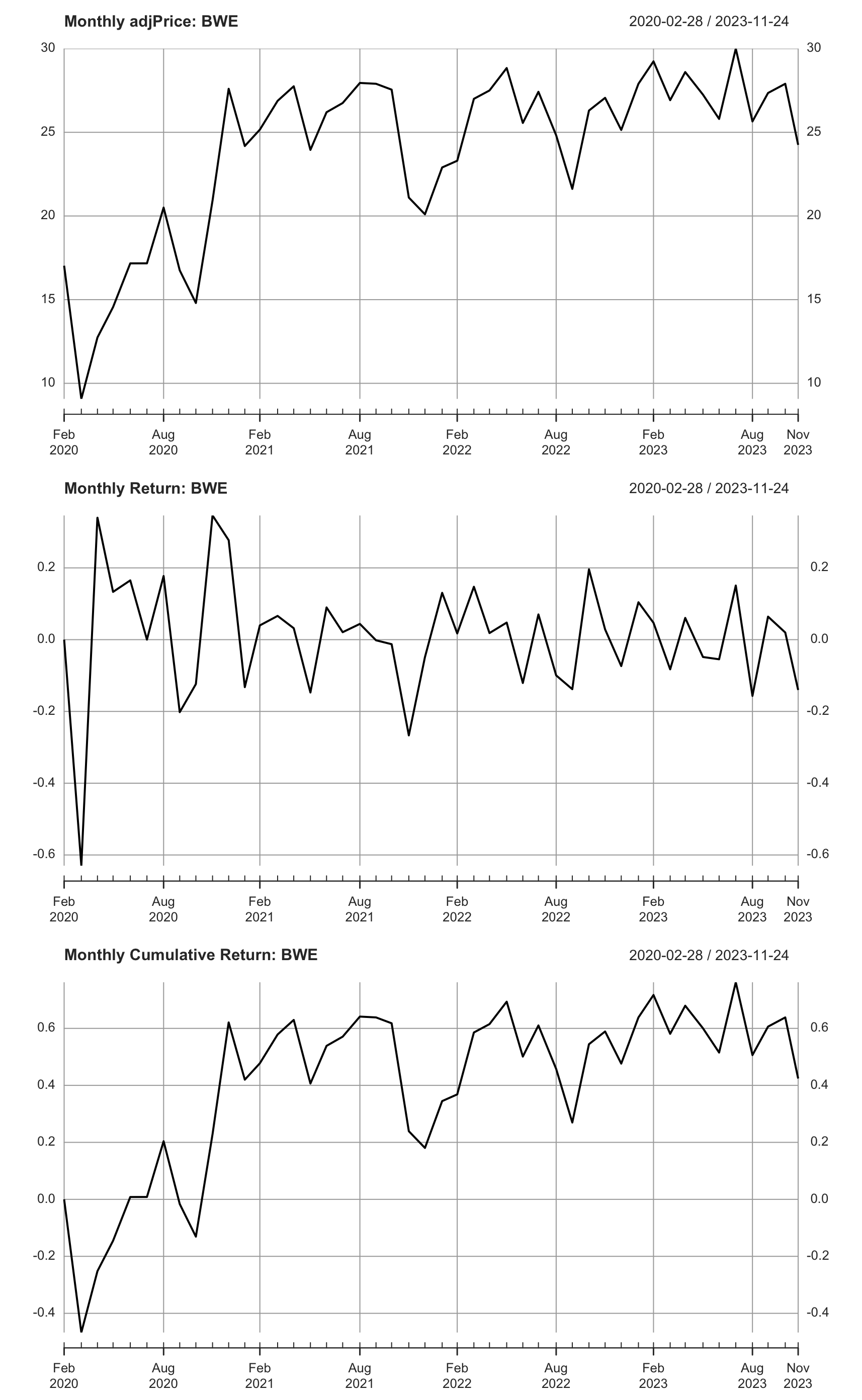
Fig. 2: Log returns
The two types act very differently when it comes to aggregation. Each has an advantage over the other:
simple returns aggregate across assets
The simple return of a portfolio is the weighted sum of the simple returns of the constituents of the portfolio.log returns aggregate across time
The log return for a time period is the sum of the log returns of partitions of the time period. For example, the log return for a year is the sum of the log returns of the days within the year.
Multiperiod returns
Multiperiod returns are the generalized case of cumulative return by allowing any holding period \(k\le T\).
The \(k\)-period (assuming annual frequency for now) simple return from time \(t-k\) to \(t\) is given by
\[ r_{t}(k) = \frac{P_t-P_{t-k}}{P_{t-k}}. \]
It can be expressed as in terms of one-period returns as follows:
\[ \begin{aligned} r_t(k) &= \prod_{j=0}^{k-1}(1+r_{t-j}) -1 \\ &= (1+r_t)(1+r_{t-1})\cdots (1+r_{t-k+1})-1 . \end{aligned} \]
We always like to talk in terms of annual performance as people like to know how much they can expect to make a year in percentage terms. That is why in most of the fund reports, you will find a standard metric called annualized returns. It is also known as the Compound Annual Growth Rate (CAGR) or the Geometric Annual Return.
Annualized return under simple returns, \(r_t^A\), is given by:
\[ \begin{split} (1+r_t^A)^k &= 1+r_t(k) \\ r_t^A &= \big(1+r_t(k) \big)^{\frac{1}{k}}-1 = \left[\prod_{j=1}^{k-1}(1+r_{t-j})\right]^{\frac{1}{k}}-1 . \end{split} \]
The \(k\)-period log return is given by
\[ z_t(k) = \ln \frac{P_t}{P_{t-k}}. \]
It is the sum of the \(k\) one-period log returns:
\[ z_t(k) = \sum_{j=0}^{k-1} z_{t-j} = z_t + z_{t-1} + \cdots + z_{t-k+1} \]
Annualized return under continuously compounding, \(z_t^A\), is given by:
\[ \begin{aligned} k\,z_t^A &= z_t(k) \\ z_t^A &= \frac{1}{k}z_t(k) = \frac{1}{k} \sum_{j=0}^{k-1} z_{t-j}, \end{aligned} \] which is the average one-period log returns.
To summarize in one table
| Simple returns | Log returns | Back out simple returns | |
|---|---|---|---|
| Single period | \(r_t=\frac{P_t}{P_{t-1}}-1\) | \(z_t=\ln \frac{P_t}{P_{t-1}}\) | \(r_t = \exp(z_t)-1\) |
| Multiperiod | \(r_t(k) = \prod_{j=0}^{k-1}(1+r_{t-j}) -1\) | \(z_t(k) = \sum_{j=0}^{k-1} z_{t-j}\) | \(r_t(k) = \exp\big(z_t(k)\big)-1\) |
| Annualized | \(r_t^A = \left[\prod_{j=0}^{k-1}(1+r_{t-j})\right]^{\frac{1}{k}}-1\) | \(z_t^A = \frac{1}{k} \sum_{j=0}^{k-1} z_{t-j}\) | \(r_t^A = \exp(z_t^A)-1\) |
Note that the annualized return here assumes the single period returns are annual returns.
In case of higher frequency data than annual, i.e., daily, weekly and monthly, we have to compound by the number of periods in a year.
daily single period: \(r_t^A = \left[\prod_{j=0}^{k-1}(1+r_{t-j})\right]^{\frac{1}{k}\cdot \color{red}{252}}-1\) for simple return, \(z_t^A = \frac{252}{k} \sum_{j=0}^{k-1} z_{t-j}\) for log return.
- Note here we used \(n=252\), i.e., the number of trading days in a year. This is applied when reporting of trading strategy returns on a product with 5 market sessions per week.
- If you are calculating CAGR for FX (which is traded effectively 24/7) strategy returns for instance, it would seem fair to use \(n=365\) calendar days.
weekly \(r_t^A = \left[\prod_{j=0}^{k-1}(1+r_{t-j})\right]^{\frac{1}{k}\cdot \color{red}{52}}-1\) for simple return, \(z_t^A = \frac{52}{k} \sum_{j=0}^{k-1} z_{t-j}\) for log return.
monthly \(r_t^A = \left[\prod_{j=0}^{k-1}(1+r_{t-j})\right]^{\frac{1}{k}\cdot \color{red}{12}}-1\) for simple return, \(z_t^A = \frac{12}{k} \sum_{j=0}^{k-1} z_{t-j}\) for log return.
quarterly \(r_t^A = \left[\prod_{j=0}^{k-1}(1+r_{t-j})\right]^{\frac{1}{k}\cdot \color{red}{4}}-1\) for simple return, \(z_t^A = \frac{4}{k} \sum_{j=0}^{k-1} z_{t-j}\) for log return.
Portfolio Returns
Consider a buy-and-hold portfolio invested in \(k\) different assets. The value at time \(t\) is
\[ V_t = \sum_{i=1}^k n_i P_{i,t} \] where \(n_i\) is the number of shares invested in asset \(i\).
Buy-and-hold portfolio: Portfolio weights from the initial portfolio are allowed to change over time as prices of the underlying assets change over time. In this case no rebalancing of the portfolio is done. \(n_i\) is constant for each asset \(i\) over the holding period. The weight increases if an asset’s price increases, and decreases otherwise. This strategy is passive and does not trade further except for the initial asset allocation.
Another trading strategy is rebalancing (monthly). This is to buy and trade at the end of each rebalance period such that your portfolio aligns with your target allocation. Regularly rebalancing a portfolio ensures that the investor maintains the desired risk and return characteristics. For instance, if the weight of a particular asset class has increased significantly due to strong performance, rebalancing involves selling a portion of that asset and reinvesting the proceeds in other assets to restore the desired portfolio weight. This is a rebalanced portfolio.
The simple one-period return of the portfolio is a weighted average of the returns of component stocks.
\[ r_{p,t} = \frac{V_t}{V_{t-1}}-1 = \sum_{i=1}^k w_{i,t} r_{i,t} \]
This result is useful. We can use the property to get the expected return and variance of the portfolio as:
\[ \begin{aligned} E[r_{p,t}] &= \sum_{i=1}^k w_{i,t} E[r_{i,t}] \\ \text{Var}[r_{p,t}] &= \sum_{i=1}^k\sum_{j=1}^k w_{i,t}\,w_{j,t}\,\text{Cov}(r_{i,t}, r_{j,t}) \end{aligned} \]
Proof. 2 Show \(r_{p,t} = \sum_{i=1}^k w_i r_{i,t}\).
\[ \begin{aligned} r_{p,t} &= \frac{V_t}{V_{t-1}} -1 \\ &= \frac{\sum_{i=1}^k n_iP_{i,t}}{\sum_{j=1}^k n_jP_{j,t-1}} -1 \\ &= \sum_{i=1}^k \frac{n_iP_{i,t-1}}{\sum_{j=1}^k n_jP_{j,t-1}} \cdot \frac{P_{i,t}}{P_{i,t-1}} - 1 \qquad \text{(multiply and divide by } P_{i, t-1} )\\ &= \sum_i w_{i,t} (r_{i,t}+1) -1 \\ &= \sum_i w_{i,t} r_{i,t} \qquad (w_{i,t} \text{ sums to 1}) \end{aligned} \] where \(w_{i,t}= \frac{n_iP_{i,t-1}}{\sum_{j=1}^k n_jP_{j,t-1}}\) is the weight of asset \(i\) at time \(t-1\).
\(\square\)
Note that an asset’s weight in month \(t\), \(w_{i,t}\), is decided by the ratio of the value of the asset to the portfolio value at the beginning of the period, i.e., at time \(t-1\).
This cross-sectional additivity does not apply to log returns. In stead we have:
\[ \begin{aligned} z_{p,t} &= \ln\,\left(\frac{V_t}{V_{t-1}}\right) \\ &= \ln \, \left(\frac{\sum_{i=1}^k n_iP_{i,t}}{\sum_{j=1}^k n_jP_{j,t-1}} \right) \\ &= \ln \, \left(\sum_{i=1}^k\frac{ n_iP_{i,t-1}}{\sum_{j=1}^k n_jP_{j,t-1}} \cdot \frac{P_{i,t}}{P_{i,t-1}} \right) \\ &= \ln \, \left(\sum_{i=1}^k w_{i,t} \frac{P_{i,t}}{P_{i,t-1}} \right) \\ &= \ln \, \left(\sum_{i=1}^k w_{i,t} \exp(z_{i,t}) \right) . \end{aligned} \] The log return of the portfolio is not a linear function for the log returns of the components.
Because the continuously compounded portfolio return is not a weighted average of the individual asset continuously compounded returns, the analysis of portfolios is typically performed using simple returns and not continuously compounded returns.
On the other hand, the log returns are additive when we consider the time series of returns:
\[ z_{p,t}(k) = \sum_{j=0}^{k-1} z_{p,t-j}. \] Given the expected values and the covariances of the subperiod returns, it is then easy to compute the expected value and the variance of the full period return.
In contrast, the time series additivity does not apply to simple returns.
\[ r_{p, t}(k) = \prod_{j=0}^{k-1} (1+r_{p,t-j}) -1 \]
Portfolio performance evaluation
We use a portfolio consisting of 2 assets as an example.
Return
Loop through assets to calculate monthly returns from daily price data.
# calculate monthly return
data_return <- titlon_group %>%
    group_modify( ~{
        xts(.$AdjustedPrice, order.by = .$Date) %>%
            to.monthly(indexAt="last", OHLC=FALSE) %>%
            Return.calculate() %>%
            data.frame() %>%
            rownames_to_column(var="Date")
    })  %>% ungroup()
colnames(data_return)[3] <- "Return_monthly"
data_return
## # A tibble: 30,351 × 3
## ISIN Date Return_monthly
## <chr> <chr> <dbl>
## 1 AU000000CSS3 2021-05-31 NA
## 2 AU000000CSS3 2021-06-30 -0.01470588
## 3 AU000000CSS3 2021-07-29 0.07462687
## 4 AU000000CSS3 2021-08-30 0.2083333
## 5 AU000000CSS3 2021-09-30 -0.1954023
## 6 AU000000CSS3 2021-10-29 0.1142857
## 7 AU000000CSS3 2021-11-29 -0.0001282051
## 8 AU000000CSS3 2021-12-29 -0.06398256
## 9 AU000000CSS3 2022-01-24 -0.01931507
## 10 AU000000CSS3 2022-02-28 0.003492108
## # ℹ 30,341 more rows## equity identifiers, ensure one-to-one mapping
select <- dplyr::select
unique_id <- titlon_data %>%
distinct(ISIN, .keep_all = TRUE) %>%
select(all_of(c("SecurityId", "CompanyId", "Symbol", "ISIN",
"Name", "Sector")))
unique_id## # A tibble: 501 × 6
## SecurityId CompanyId Symbol ISIN Name
## <dbl> <dbl> <chr> <chr> <chr>
## 1 1304857 12720 2020 BMG9156K1018 2020 Bulkers
## 2 1301972 12440 FIVEPG DK0060945467 5th Planet Games
## 3 NA NA AASB NO0010672181 Aasen Sparebank
## 4 6085 2017 ABG NO0003021909 ABG Sundal Collier
## 5 1301198 12348 ABL NO0010715394 ABL GROUP
## 6 1304655 12701 ADE NO0010844038 Adevinta
## 7 1304652 12701 ADEA NO0010843998 Adevinta ser. A
## 8 NA NA ADS CY0108052115 ADS Crude Carriers
## 9 1251504 11273 AEGA NO0010626559 Aega
## 10 NA NA AEGA NO0012958539 AEGA
## Sector
## <chr>
## 1 Industrials
## 2 Consumer Discretionary
## 3 Financials
## 4 Financials
## 5 Industrials
## 6 Consumer Discretionary
## 7 Consumer Discretionary
## 8 Industrials
## 9 Financials
## 10 Financials
## # ℹ 491 more rows## add company info
data_return <- data_return %>%
left_join(unique_id, by="ISIN") %>%
select("ISIN", "Date",
"Symbol", "Name", "Sector",
"Return_monthly")
## subset complete cases
start_date <- ymd("2015-01-01")
end_date <- ymd("2022-12-31")
data_return <- data_return %>%
mutate(Date = ymd(Date)) %>%
filter(between(Date, start_date, end_date))
ISIN_vec <- data_return %>% group_by(ISIN) %>%
tally(sort=TRUE) %>%
filter(n==96) %>%
pull(ISIN)
ISIN_vec %>% length() # 142 complete cases## [1] 142data_return <- data_return %>% filter(ISIN %in% ISIN_vec)
data_return## # A tibble: 13,632 × 6
## ISIN Date Symbol Name Sector Return_monthly
## <chr> <date> <chr> <chr> <chr> <dbl>
## 1 BMG0451H1170 2015-01-30 ARCHER Archer Energy -0.2400990
## 2 BMG0451H1170 2015-02-27 ARCHER Archer Energy -0.2280130
## 3 BMG0451H1170 2015-03-31 ARCHER Archer Energy 0.008438819
## 4 BMG0451H1170 2015-04-30 ARCHER Archer Energy 0.1673640
## 5 BMG0451H1170 2015-05-29 ARCHER Archer Energy -0.03942652
## 6 BMG0451H1170 2015-06-30 ARCHER Archer Energy 0.007462687
## 7 BMG0451H1170 2015-07-31 ARCHER Archer Energy -0.2148148
## 8 BMG0451H1170 2015-08-31 ARCHER Archer Energy -0.4009434
## 9 BMG0451H1170 2015-09-30 ARCHER Archer Energy -0.1299213
## 10 BMG0451H1170 2015-10-30 ARCHER Archer Energy -0.07692308
## # ℹ 13,622 more rowsGet sample data for two assets and create an equally-weighted portfolio of them.
k <- 2 # number of asset
sample_data <- data_return %>%
    filter(ISIN %in% c("BMG0451H1170", "NO0003079709"))
sample_data
## # A tibble: 192 × 6
## ISIN Date Symbol Name Sector Return_monthly
## <chr> <date> <chr> <chr> <chr> <dbl>
## 1 BMG0451H1170 2015-01-30 ARCHER Archer Energy -0.2400990
## 2 BMG0451H1170 2015-02-27 ARCHER Archer Energy -0.2280130
## 3 BMG0451H1170 2015-03-31 ARCHER Archer Energy 0.008438819
## 4 BMG0451H1170 2015-04-30 ARCHER Archer Energy 0.1673640
## 5 BMG0451H1170 2015-05-29 ARCHER Archer Energy -0.03942652
## 6 BMG0451H1170 2015-06-30 ARCHER Archer Energy 0.007462687
## 7 BMG0451H1170 2015-07-31 ARCHER Archer Energy -0.2148148
## 8 BMG0451H1170 2015-08-31 ARCHER Archer Energy -0.4009434
## 9 BMG0451H1170 2015-09-30 ARCHER Archer Energy -0.1299213
## 10 BMG0451H1170 2015-10-30 ARCHER Archer Energy -0.07692308
## # ℹ 182 more rowsret_mat <- sample_data %>% pull(Return_monthly) %>%
matrix(ncol=k)
ret_mat %>% dim()## [1] 96 2wts <- rep(1/k, k)
wts## [1] 0.5 0.5Calculate portfolio return manually (most concise). It is straightforward to calculate rebalanced, as the begin of period weights are always the same. But it is a bit cumbersome to calculate buy-and-hold as we need to update the weight for each period.
Here shows an example of rebalancing monthly.
# option 1, matrix representation
ptf_ret <- ret_mat %*% matrix(wts, ncol=1)
names(ptf_ret) <- "port_ret_manual"
ptf_ret %>% head(10)
## [,1]
## [1,] -0.122990026
## [2,] -0.043001570
## [3,] 0.022356632
## [4,] 0.247278035
## [5,] 0.003363661
## [6,] -0.036708697
## [7,] -0.007408891
## [8,] -0.253805031
## [9,] -0.061228133
## [10,] 0.081909129Alternatively, we can use PerformanceAnalytics package. It provides many functions convenient for performance evaluation. We need to convert the data to xts before providing it as the input for PerformanceAnalytics functions.
## using PerformanceAnalytics::Return.portfolio
sample_data <- sample_data %>%      # standardize date
    mutate(yrmon=as.yearmon(Date))
sample_data <- sample_data %>%
    mutate(Date=as.Date(yrmon, frac=1))
return_xts <- sample_data %>% pull(Return_monthly) %>%
    matrix(ncol=k) %>%
    xts(order.by = sample_data$Date %>% unique())
colnames(return_xts) <- sample_data$Symbol %>% unique()
return_xts %>% str()
## An xts object on 2015-01-31 / 2022-12-31 containing:
## Data: double [96, 2]
## Columns: ARCHER, KIT
## Index: Date [96] (TZ: "UTC")return_xts %>%
data.frame %>%
knitr::kable(digits = 5, caption = "Component asset monthly returns") %>%
kable_styling(bootstrap_options = c("striped", "hover"), full_width = F, latex_options="scale_down") %>%
scroll_box(height = "500px")| ARCHER | KIT | |
|---|---|---|
| 2015-01-31 | -0.24010 | -0.00588 |
| 2015-02-28 | -0.22801 | 0.14201 |
| 2015-03-31 | 0.00844 | 0.03627 |
| 2015-04-30 | 0.16736 | 0.32719 |
| 2015-05-31 | -0.03943 | 0.04615 |
| 2015-06-30 | 0.00746 | -0.08088 |
| 2015-07-31 | -0.21481 | 0.20000 |
| 2015-08-31 | -0.40094 | -0.10667 |
| 2015-09-30 | -0.12992 | 0.00746 |
| 2015-10-31 | -0.07692 | 0.24074 |
| 2015-11-30 | -0.16176 | 0.06567 |
| 2015-12-31 | -0.27485 | 0.09244 |
| 2016-01-31 | -0.27419 | 0.05128 |
| 2016-02-29 | -0.40667 | -0.02683 |
| 2016-03-31 | 0.80899 | 0.08772 |
| 2016-04-30 | 0.46998 | 0.07126 |
| 2016-05-31 | -0.09296 | 0.00899 |
| 2016-06-30 | -0.16149 | -0.01114 |
| 2016-07-31 | -0.11111 | 0.26126 |
| 2016-08-31 | -0.17292 | -0.03036 |
| 2016-09-30 | 0.20907 | 0.01289 |
| 2016-10-31 | 0.40000 | 0.01273 |
| 2016-11-30 | -0.04167 | 0.08618 |
| 2016-12-31 | 0.95652 | -0.00331 |
| 2017-01-31 | 0.30159 | 0.10448 |
| 2017-02-28 | -0.29878 | 0.08108 |
| 2017-03-31 | 0.18261 | -0.09444 |
| 2017-04-30 | -0.04412 | 0.09618 |
| 2017-05-31 | -0.12692 | 0.04499 |
| 2017-06-30 | -0.13833 | 0.10000 |
| 2017-07-31 | 0.18098 | 0.11742 |
| 2017-08-31 | -0.14545 | -0.07684 |
| 2017-09-30 | 0.21581 | -0.01469 |
| 2017-10-31 | -0.18833 | -0.11553 |
| 2017-11-30 | -0.13860 | 0.01124 |
| 2017-12-31 | 0.19785 | -0.02917 |
| 2018-01-31 | 0.04876 | 0.18026 |
| 2018-02-28 | -0.12334 | 0.03636 |
| 2018-03-31 | -0.12662 | 0.01754 |
| 2018-04-30 | 0.16481 | 0.10216 |
| 2018-05-31 | 0.15319 | 0.07301 |
| 2018-06-30 | -0.01292 | 0.01134 |
| 2018-07-31 | -0.14486 | -0.03466 |
| 2018-08-31 | -0.21749 | 0.03485 |
| 2018-09-30 | 0.06145 | -0.00306 |
| 2018-10-31 | -0.07895 | -0.12590 |
| 2018-11-30 | -0.12286 | 0.04684 |
| 2018-12-31 | -0.29235 | -0.02685 |
| 2019-01-31 | 0.08631 | -0.01149 |
| 2019-02-28 | 0.17797 | 0.03488 |
| 2019-03-31 | -0.11151 | -0.02247 |
| 2019-04-30 | 0.12348 | 0.10345 |
| 2019-05-31 | -0.28649 | -0.04996 |
| 2019-06-30 | 0.14394 | 0.05263 |
| 2019-07-31 | 0.02980 | 0.11087 |
| 2019-08-31 | -0.10825 | -0.07045 |
| 2019-09-30 | -0.05529 | -0.02526 |
| 2019-10-31 | -0.11832 | 0.00864 |
| 2019-11-30 | -0.16883 | 0.00321 |
| 2019-12-31 | 0.10417 | 0.17395 |
| 2020-01-31 | -0.09119 | -0.07454 |
| 2020-02-29 | -0.01557 | 0.03144 |
| 2020-03-31 | -0.36801 | -0.18286 |
| 2020-04-30 | -0.07119 | 0.25874 |
| 2020-05-31 | 0.23653 | 0.08889 |
| 2020-06-30 | 0.04116 | 0.00510 |
| 2020-07-31 | -0.02791 | 0.26903 |
| 2020-08-31 | 0.13636 | 0.09066 |
| 2020-09-30 | -0.10947 | 0.11736 |
| 2020-10-31 | 0.01182 | -0.03241 |
| 2020-11-30 | 0.44626 | -0.04593 |
| 2020-12-31 | -0.00646 | 0.03899 |
| 2021-01-31 | 0.36098 | -0.10265 |
| 2021-02-28 | -0.06810 | 0.04551 |
| 2021-03-31 | 0.11923 | 0.29411 |
| 2021-04-30 | 0.19817 | -0.07088 |
| 2021-05-31 | -0.13193 | 0.08707 |
| 2021-06-30 | 0.02423 | -0.09108 |
| 2021-07-31 | -0.05699 | -0.02115 |
| 2021-08-31 | -0.09920 | -0.01440 |
| 2021-09-30 | 0.24051 | -0.05219 |
| 2021-10-31 | -0.01020 | 0.00906 |
| 2021-11-30 | -0.21237 | 0.07016 |
| 2021-12-31 | 0.00000 | 0.22789 |
| 2022-01-31 | 0.11257 | -0.04025 |
| 2022-02-28 | -0.23294 | -0.08168 |
| 2022-03-31 | 0.01227 | -0.03125 |
| 2022-04-30 | -0.10606 | -0.06995 |
| 2022-05-31 | 0.36441 | 0.02489 |
| 2022-06-30 | -0.13043 | -0.07392 |
| 2022-07-31 | 0.01429 | 0.18871 |
| 2022-08-31 | 0.08310 | -0.03837 |
| 2022-09-30 | -0.14174 | -0.06135 |
| 2022-10-31 | 0.11515 | 0.23805 |
| 2022-11-30 | 0.00136 | 0.01073 |
| 2022-12-31 | -0.06649 | 0.19108 |
Return.portfolio can do buy-and-hold and rebalanced strategies rather easily.
We do not need to calculate the weight on our own in case of buy-and-hold.
# buy and hold ptf
ptf_bh <- Return.portfolio(R = return_xts, weights = wts, verbose = TRUE)
# rebalanced ptf
ptf_rebal <- Return.portfolio(R = return_xts, weights = wts, rebalance_on="month", verbose = TRUE)
Plot the portfolio monthly returns.
plot_data <- ptf_bh$returns %>%
    merge(ptf_rebal$returns) %>%
    setNames(c("buy-and-hold", "rebalance"))
plot(plot_data, multi.panel=TRUE, main="Portfolio monthly return")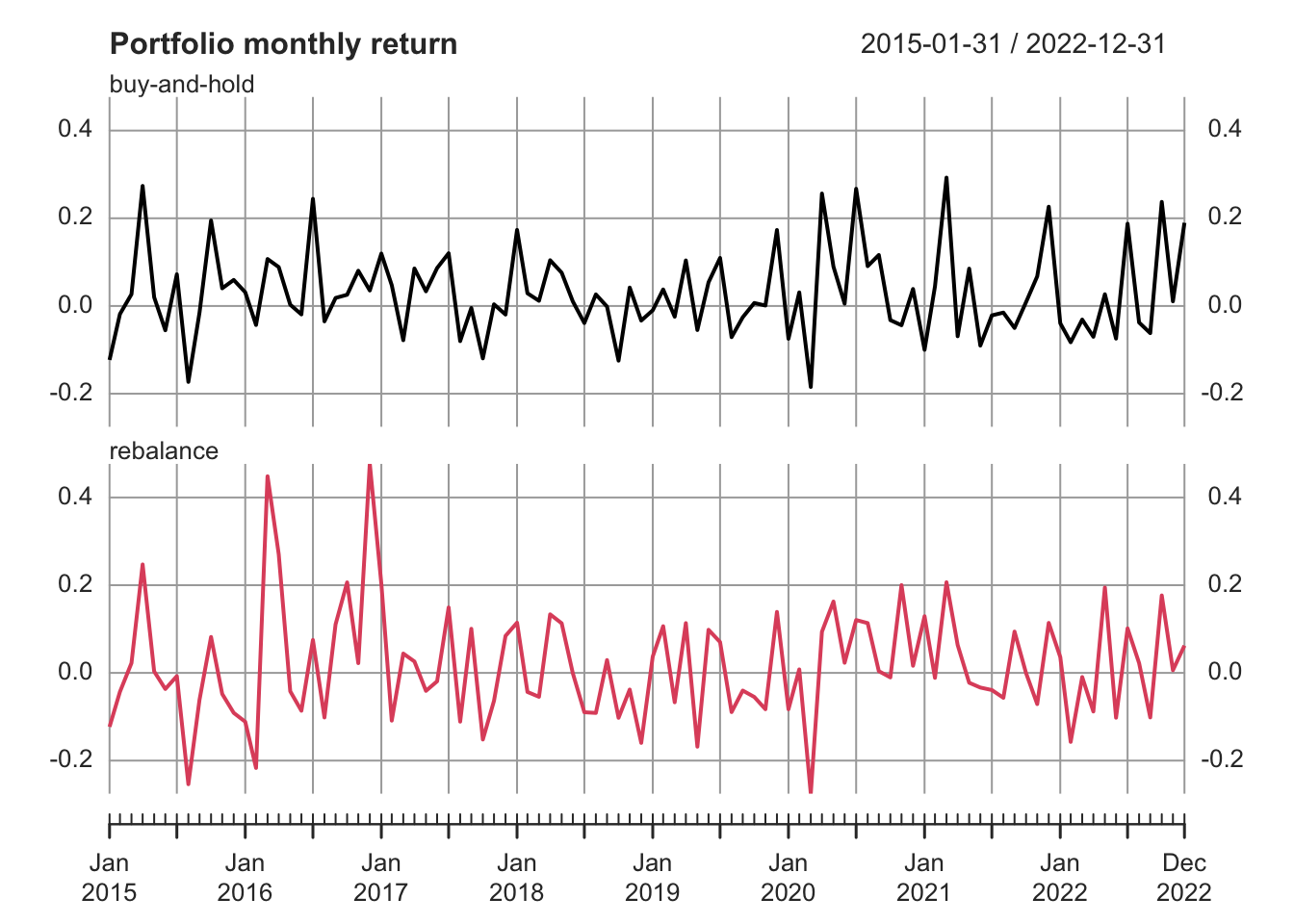
Plot the portfolio cumulative returns.
plot_data <- ptf_bh$returns %>%
    merge(ptf_rebal$returns) %>%
    as_tibble() %>%
    mutate_all(~cumprod(1+.)) %>%
    xts(order.by = index(ptf_bh$returns)) %>%
    setNames(c("buy-and-hold", "rebalance"))
plot(plot_data, multi.panel=TRUE, main="Portfolio cumulative return", yaxis.same=FALSE)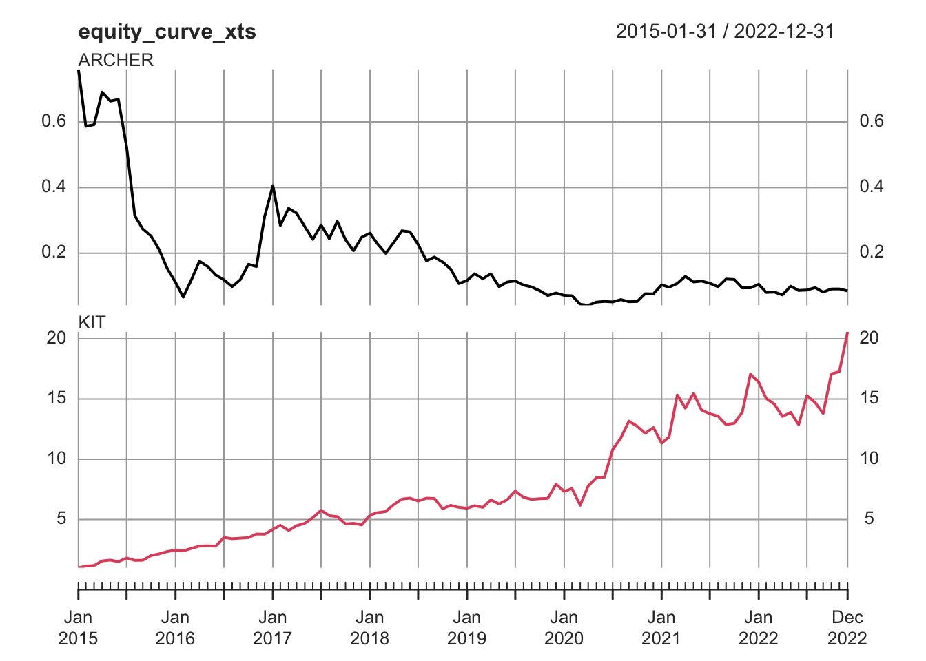
By setting verbose = TRUE, it allows us to check intermediary calculations, such as contributions, weight for each asset.
Here we check the end of period weight.
# plot end of period weights
eop_weight_bh <- ptf_bh$EOP.Weight
eop_weight_rebal <- ptf_rebal$EOP.Weight
par(mfrow = c(2, 1), mar = c(2, 4, 2, 2))
plot.xts(eop_weight_bh$KIT)
plot.xts(eop_weight_rebal$KIT)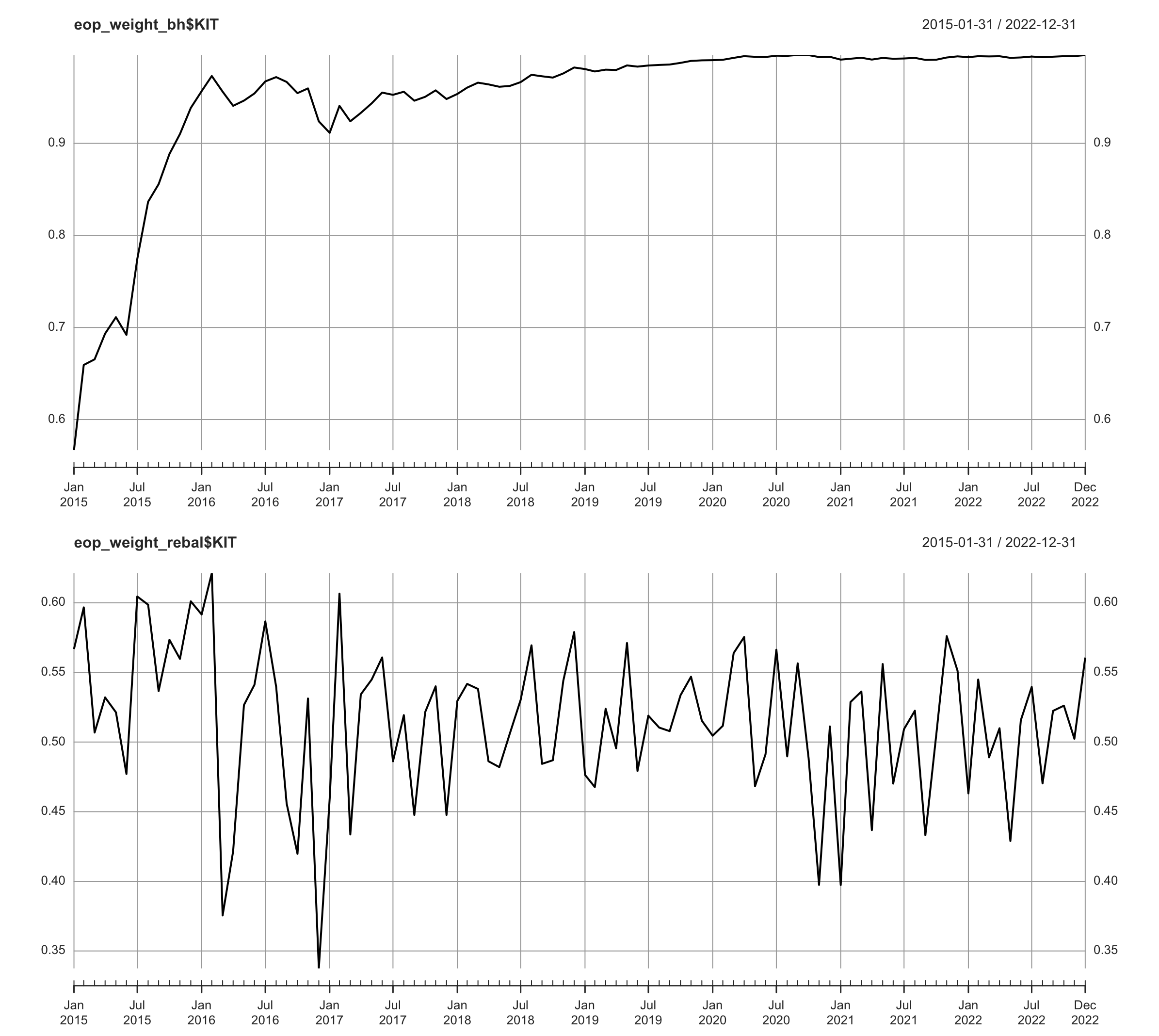
Fig. 3: Weight of KIT under buy-and-hold and rebalancing.
We see that the weight of KIT basically skyrockets and dominates the portfolio, taking up more than \(99\%\) of the portfolio.
This is due to its strong performance.
Now we check the relative performance of the two assets.
## check relative performance by calculating the equity curve
equity_curve_xts <- return_xts %>%
    apply(2, function(col) cumprod(1 + col))
equity_curve_xts <- xts(equity_curve_xts, index(return_xts))
colnames(equity_curve_xts) <- colnames(return_xts)
plot(equity_curve_xts, multi.panel=TRUE, yaxis.same=FALSE)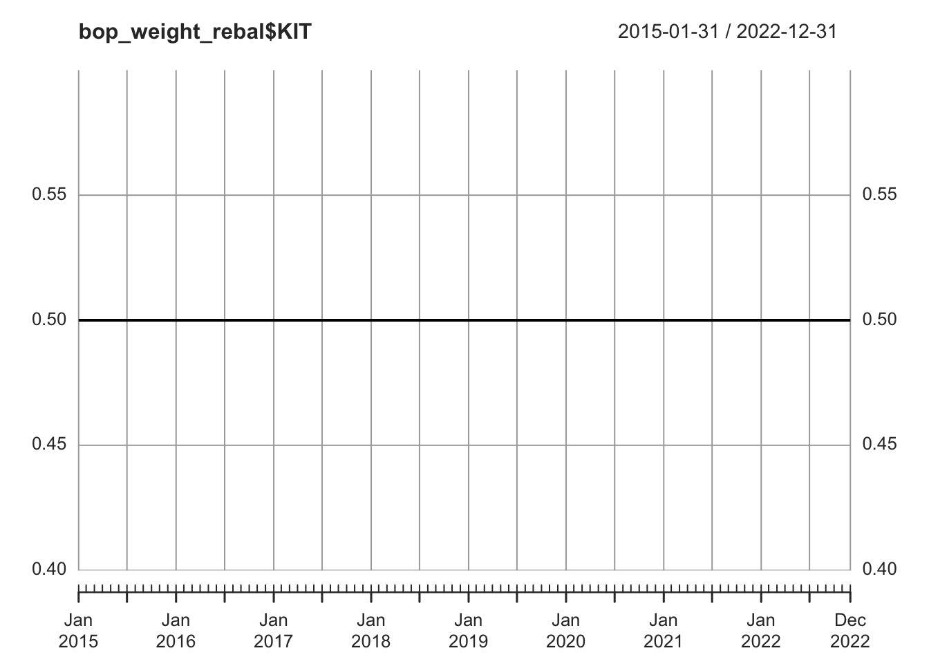
Portfolio performance attribution aggregated by year
ptf_bh$contribution %>%
    to.period.contributions(period = "years") %>%
    data.frame() %>%
    knitr::kable(digits = 4, caption = "portfolio performance attribution") %>%
kable_styling(bootstrap_options = c("striped", "hover"), full_width = F, latex_options="scale_down")| ARCHER | KIT | Portfolio.Return | |
|---|---|---|---|
| 2015-12-31 | -0.4233 | 0.6711 | 0.2478 |
| 2016-12-31 | 0.0635 | 0.5775 | 0.6410 |
| 2017-12-31 | -0.0154 | 0.1870 | 0.1716 |
| 2018-12-31 | -0.0294 | 0.3036 | 0.2742 |
| 2019-12-31 | -0.0047 | 0.3138 | 0.3091 |
| 2020-12-31 | -0.0003 | 0.5881 | 0.5878 |
| 2021-12-31 | 0.0015 | 0.3493 | 0.3507 |
| 2022-12-31 | -0.0005 | 0.2042 | 0.2036 |
Q: What does the begin of period weight look like?
A: A horizontal line at \(y=50\%\).
bop_weight_rebal <- ptf_rebal$BOP.Weight
plot(bop_weight_rebal$KIT)
Now we build an equal-weighted portfolio consisting of 10 stocks per period, rebalanced annually. Then compute and plot portfolio returns using PerformanceAnalytics. This is useful when you backtest a trading strategy.
# Backtest a hypothetical trading strategy
# Define list of selected symbols for each year (2015 to 2022, 8 yrs)
selected_symbol_by_year <- list(
  c("AURG", "RISH", "SADG", "HBC", "AKVA", "NONG", "ENTRA", "YAR", "PGS", "BMA"),
  c("YAR", "AKER", "APP", "XXL", "MSEIS", "ABL", "PSI", "RISH", "SALM", "WWI"),
  c("ATEA", "MELG", "AMSC", "KOG", "BLO", "SBVG", "ODFB", "NKR", "JAEREN", "ZAL"),
  c("ODL", "KOA", "DLTX", "NHY", "ENTRA", "KOG", "PROT", "AFG", "NAVA", "SOR"),
  c("EQNR", "DNO", "SOAG", "VVL", "KIT", "BAKKA", "WAWI", "DLTX", "AXA", "ROM"),
  c("FRO", "PHO", "DNO", "ZAL", "APP", "NHY", "MGN", "IOX", "KOA", "GJF"),
  c("RING", "GSF", "PCIB", "ABG", "VEI", "ABT", "AKPS", "SUBC", "PGS", "SAGA"),
  c("SBX", "ODF", "OPERA", "PEN", "SKUE", "SAGA", "HELG", "NOM", "MHG", "NONG")
  )
returns_xts <- data_return %>%
    select(Date, Symbol, Return_monthly) %>%
    mutate(Date = as.Date(as.yearmon(Date), frac=1)) %>%  # standardize end of month date
    spread(key=Symbol, value=Return_monthly)
returns_xts <- returns_xts %>% xts(x=.[,-1], order.by=.[[1]])

# Construct weights xts object
dates <- index(returns_xts)
weights_list <- list()

for (i in 1:8) {
  year_start <- as.Date(paste0(2014 + i, "-01-01"))
  year_end <- as.Date(paste0(2014 + i, "-12-31"))
  period_dates <- dates[dates >= year_start & dates <= year_end]

  weights <- matrix(0, nrow = length(period_dates), ncol = ncol(returns_xts))
  colnames(weights) <- colnames(returns_xts)

  valid_symbols <- colnames(returns_xts) %in% selected_symbol_by_year[[i]]
  weights[, valid_symbols] <- 1 / 10

  weights_xts <- xts(weights, order.by = period_dates)
  weights_list[[i]] <- weights_xts
}

# Combine weights into one xts object
final_weights_xts <- do.call(rbind, weights_list)

# Align weights and returns
aligned_weights <- final_weights_xts[index(returns_xts)]

# Calculate portfolio return
portfolio_return <- Return.portfolio(R = returns_xts,
                                     weights = aligned_weights,
                                     verbose = TRUE)
Plot portfolio returns.
charts.PerformanceSummary(portfolio_return$returns)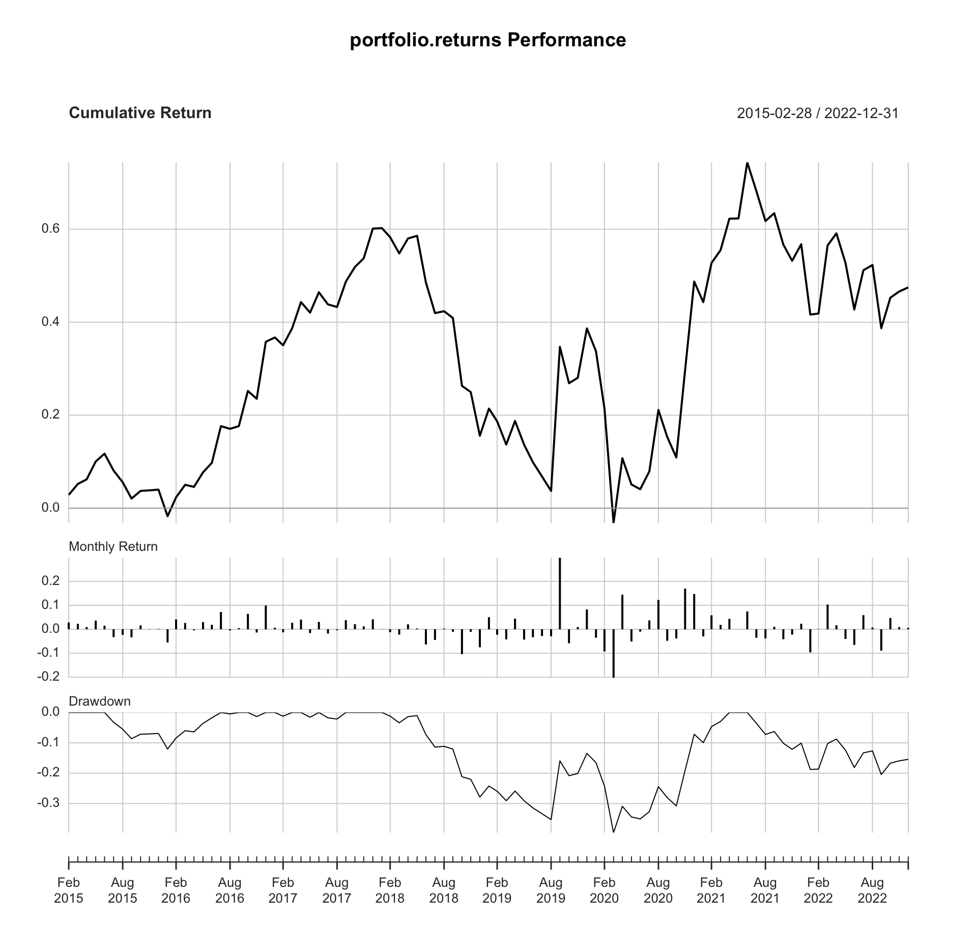
Fig. 4: Portfolio performance.
Overall performance
# summary statistics
table.AnnualizedReturns(portfolio_return$returns) %>%
    knitr::kable(digits = 4, caption = "Overall performance") %>%
kable_styling(bootstrap_options = c("striped", "hover"), full_width = F, latex_options="scale_down")| portfolio.returns | |
|---|---|
| Annualized Return | 0.0503 |
| Annualized Std Dev | 0.2184 |
| Annualized Sharpe (Rf=0%) | 0.2304 |
Performance by year
# Split portfolio return by year
portfolio_by_year <- split.xts(portfolio_return$returns, f = "years")

# Calculate annualized returns by year
library(moments)  # for skewness and kurtosis
performance_metrics <- function(x) {
  ann_ret <- table.AnnualizedReturns(x)
  skew <- skewness(na.omit(x))
  kurt <- kurtosis(na.omit(x))
  max_dd <- maxDrawdown(x)  # Maximum Drawdown
  var_95 <- VaR(x, p = 0.95, method = "historical")  # Value at Risk (VaR)
  # Conditional VaR (CVaR) / Expected Shortfall
  cvar_95 <- CVaR(x, p = 0.95, method = "historical")
  sortino <- SortinoRatio(x)

  # Combine metrics
  out <- rbind(ann_ret,
               Skewness = skew,
               Kurtosis = kurt,
               MaxDrawdown = max_dd,
               VaR_95 = var_95,
               CVaR_95 = cvar_95,
               SortinoRatio = sortino)
  return(out)
}
metrics_by_year <- lapply(portfolio_by_year, performance_metrics)
metrics_by_year$all <- performance_metrics(portfolio_return$returns)
# Combine results into a single table
annualized_table <- do.call(cbind, metrics_by_year)
colnames(annualized_table) <- names(metrics_by_year)

# Print the table
annualized_table %>%
    knitr::kable(digits = 4, caption = "Performance by year") %>%
kable_styling(bootstrap_options = c("striped", "hover"), full_width = F, latex_options="scale_down")| 2015 | 2016 | 2017 | 2018 | 2019 | 2020 | 2021 | 2022 | all | |
|---|---|---|---|---|---|---|---|---|---|
| Annualized Return | 0.0437 | 0.3058 | 0.1792 | -0.2782 | 0.1997 | 0.0727 | 0.0539 | -0.0592 | 0.0503 |
| Annualized Std Dev | 0.0834 | 0.1463 | 0.0775 | 0.1298 | 0.3411 | 0.3950 | 0.1373 | 0.2084 | 0.2184 |
| Annualized Sharpe (Rf=0%) | 0.5236 | 2.0903 | 2.3116 | -2.1428 | 0.5855 | 0.1841 | 0.3925 | -0.2840 | 0.2304 |
| Skewness | -0.4463 | 0.0641 | -0.1940 | -0.8216 | 2.0704 | -0.1066 | 0.3603 | -0.0543 | 1.0100 |
| Kurtosis | 1.9204 | 2.5794 | 1.5451 | 2.5507 | 6.5651 | 2.1599 | 1.8566 | 2.2475 | 8.0514 |
| MaxDrawdown | 0.0865 | 0.0550 | 0.0216 | 0.2787 | 0.1459 | 0.3019 | 0.1214 | 0.1282 | 0.3959 |
| VaR_95 | -0.0330 | -0.0322 | -0.0167 | -0.0879 | -0.0499 | -0.1421 | -0.0396 | -0.0924 | -0.0793 |
| CVaR_95 | -0.0333 | -0.0550 | -0.0178 | -0.1036 | -0.0581 | -0.2027 | -0.0413 | -0.0964 | -0.1169 |
| SortinoRatio | 0.2442 | 1.4141 | 1.8012 | -0.5943 | 0.6569 | 0.1717 | 0.2316 | -0.0774 | 0.1644 |
Risk-adjusted returns
Excess return and Sharpe ratio.
## load risk free and market rates
f_name <- "data/NO_Rf-OSEBX_2015-2023_monthly.csv"
rfr <- read_csv(f_name)
rfr <- rfr %>% mutate(yrmon=as.yearmon(Date))
ptf_ret3 <- ptf_rebal$returns %>%
    data.frame(row.names = index(ptf_bh$returns)) %>%
    as_tibble(rownames="Date") %>%
    mutate(yrmon=as.yearmon(Date))
bind_cols(ptf_ret, ptf_ret3) # cross validate hand and computer calculations
## # A tibble: 96 × 4
## ...1 Date portfolio.returns yrmon
## <dbl> <chr> <dbl> <yearmon>
## 1 -0.1229900 2015-01-31 -0.1229900 Jan 2015
## 2 -0.04300157 2015-02-28 -0.04300157 Feb 2015
## 3 0.02235663 2015-03-31 0.02235663 Mar 2015
## 4 0.2472780 2015-04-30 0.2472780 Apr 2015
## 5 0.003363661 2015-05-31 0.003363661 May 2015
## 6 -0.03670870 2015-06-30 -0.03670870 Jun 2015
## 7 -0.007408891 2015-07-31 -0.007408891 Jul 2015
## 8 -0.2538050 2015-08-31 -0.2538050 Aug 2015
## 9 -0.06122813 2015-09-30 -0.06122813 Sep 2015
## 10 0.08190913 2015-10-31 0.08190913 Oct 2015
## # ℹ 86 more rowsMerge with risk free rate.
colnames(ptf_ret3)[2] <- "port_ret"
ptf_ret3 <- ptf_ret3 %>%
    left_join(rfr[,-1], by="yrmon") %>%
    mutate(excess_ret = port_ret-rf_1month)
ptf_ret3
## # A tibble: 96 × 7
## Date port_ret yrmon mkt_return_monthly rf_1month rf_annualized
## <chr> <dbl> <yearmon> <dbl> <dbl> <dbl>
## 1 2015-01-31 -0.1229900 Jan 2015 0.03498025 0.0012 0.01449542
## 2 2015-02-28 -0.04300157 Feb 2015 0.03262385 0.00113 0.01364459
## 3 2015-03-31 0.02235663 Mar 2015 0.005782596 0.00127 0.01534690
## 4 2015-04-30 0.2472780 Apr 2015 0.03255810 0.00123 0.01486026
## 5 2015-05-31 0.003363661 May 2015 0.009884897 0.00117 0.01413070
## 6 2015-06-30 -0.03670870 Jun 2015 -0.02566288 0.00102 0.0123089
## 7 2015-07-31 -0.007408891 Jul 2015 0.01560936 0.00097 0.01170230
## 8 2015-08-31 -0.2538050 Aug 2015 -0.07016421 0.00095 0.01145975
## 9 2015-09-30 -0.06122813 Sep 2015 -0.02072041 0.00083 0.01000559
## 10 2015-10-31 0.08190913 Oct 2015 0.05749500 0.0008 0.009642353
## excess_ret
## <dbl>
## 1 -0.1241900
## 2 -0.04413157
## 3 0.02108663
## 4 0.2460480
## 5 0.002193661
## 6 -0.03772870
## 7 -0.008378891
## 8 -0.2547550
## 9 -0.06205813
## 10 0.08110913
## # ℹ 86 more rows# Portfolio performance relative to benchmark
ptf_ret3[, c("Date", "port_ret", "mkt_return_monthly")] %>%
mutate(Date = ymd(Date)) %>%
xts(x=.[,-1], order.by=.[[1]]) %>%
charts.PerformanceSummary(main = "Portfolio performance relative to benchmark")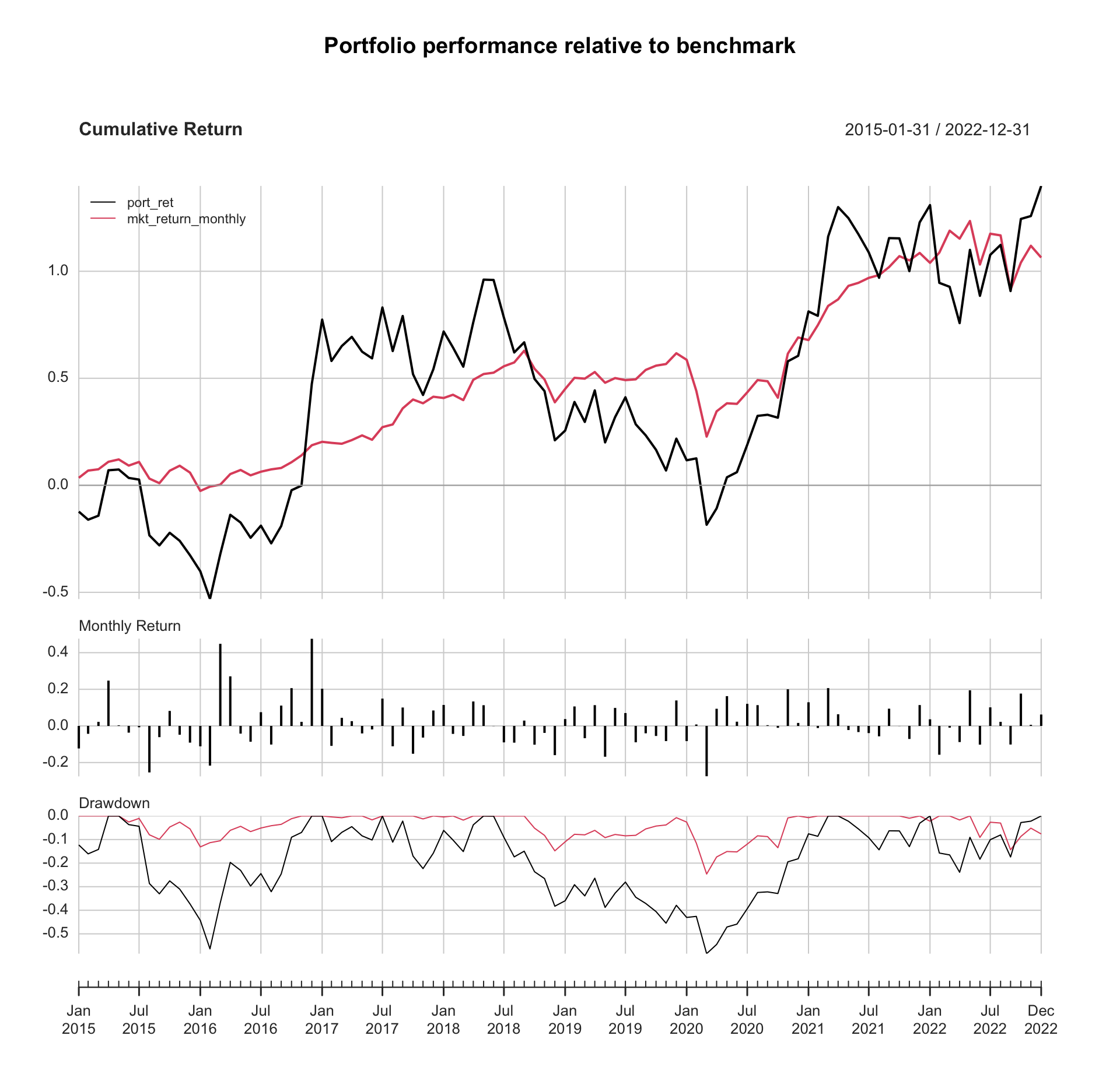
Monthly mean and volatility
- Arithmetic mean (AM) portfolio return \(\bar{r}_{p, 0:T}\)
\[ \text{Arithmetic } \bar{r}_{p, 0:T} = \frac{\sum_{t=1}^T r_{p,t}}{T} \]
Geometric mean (GM) portfolio return
\[ \text{Geometric } \bar{r}_{p, 0:T} = \left[\prod_{t=1}^T (1+r_{p,t}) \right] ^{\frac{1}{T}}-1 \]
Written as \(\bar{r}_p\) in short, representing the arithmetic/geometric mean return of the portfolio from time \(0\) to time \(T\).
Arithmetic average sometimes cannot precisely reflect historical gains and losses. Suppose the original capital of \(\$100\) is invested over a two-month period with 10% return in the first month and \(10\%\) loss in the second month.
The arithmetic average return is \((10\% - 10\%)/2=0\%\), which implies that there is no change in the \(\$100\) invested. However, the actual gain/loss for the investment grows from \(\$100\) to \(\$110\) in the first month, and drops 10% from \(\$110\) to \(\$99\) in the second month, indicating an actual loss of \(\$1\).
The geometric return is \((1.1\times0.9)^{0.5}-1\approx -0.5\%\), indicating a loss of \(-0.5\%\) per month. The geometric return that incorporates the compounding effect of growth is a better indication of historical performance.
Geometric mean is smaller than or equal to arithmetic mean and the equality holds if and only if \(r_{p,1}=r_{p,2}=\cdots=r_{p,T}\). This can be proven by using Jensen’s inequality that says, for any concave function \(g(x)\),
\[ E[g(x)] \le g(E[x]). \]
And \(\ln(x)\) is a concave function.
Common practice is to report geometric mean portfolio return.
# arithmetic mean monthly returns
mean(ptf_ret3$port_ret)
## [1] 0.01681626# geometric mean
mean.geometric(ptf_ret3$port_ret) ## [1] 0.009155608prod(1+ptf_ret3$port_ret)^(1/96)-1## [1] 0.009155608# mean excess return
mean(ptf_ret3$excess_ret) ## [1] 0.01599762mean.geometric(ptf_ret3$excess_ret)## [1] 0.008326127# standard deviation
sd(ptf_ret3$port_ret)## [1] 0.1278693Portfolio return and standard deviation are usually published as annualized.
Annualized arithmetic return assuming \(r_{p,t}\) being monthly return
\[ r_{p}^A = \frac{12}{T}\sum_{t=1}^T r_{p,t} = 12\times \bar{r}_p \]
where \(\bar{r}_p\) is the arithmetic mean.
Annualized geometric return
\[ r_{p}^A = \left[\prod_{t=1}^T (1+r_{p,t}) \right]^{\frac{12}{T}}-1 = (1+\bar{r}_p)^{12}-1 \]
where \(\bar{r}_p\) is the geometric mean.
Annualized standard deviation.
Note that in Finance, the standard deviation of returns is usually called volatility.
\[ \begin{aligned} \sigma_{p}^A &= \sqrt{12} \sigma_p \\ \sigma_p^2 &= \frac{1}{T-1} \sum_{t=1}^T (r_{p,t}-\bar{r}_p)^2 \end{aligned} \]
It is possible to use Return.annualized, StdDev.annualized from the PerformanceAnalytics package to get the annualized statistics, but we need to convert the portfolio return as an xts object.
# convert portfolio return to xts object
ptf_xts <- xts(ptf_ret3[,-c(1,3)], order.by=ymd(ptf_ret3$Date))
ptf_xts %>%
    data.frame %>%
    knitr::kable(digits = 5, caption = "Portfolio return in `xts`") %>%
    kable_styling(bootstrap_options = c("striped", "hover"), full_width = F, latex_options="scale_down") %>%
scroll_box(height = "500px")| port_ret | mkt_return_monthly | rf_1month | rf_annualized | excess_ret | |
|---|---|---|---|---|---|
| 2015-01-31 | -0.12299 | 0.03498 | 0.00120 | 0.01450 | -0.12419 |
| 2015-02-28 | -0.04300 | 0.03262 | 0.00113 | 0.01364 | -0.04413 |
| 2015-03-31 | 0.02236 | 0.00578 | 0.00127 | 0.01535 | 0.02109 |
| 2015-04-30 | 0.24728 | 0.03256 | 0.00123 | 0.01486 | 0.24605 |
| 2015-05-31 | 0.00336 | 0.00988 | 0.00117 | 0.01413 | 0.00219 |
| 2015-06-30 | -0.03671 | -0.02566 | 0.00102 | 0.01231 | -0.03773 |
| 2015-07-31 | -0.00741 | 0.01561 | 0.00097 | 0.01170 | -0.00838 |
| 2015-08-31 | -0.25381 | -0.07016 | 0.00095 | 0.01146 | -0.25476 |
| 2015-09-30 | -0.06123 | -0.02072 | 0.00083 | 0.01001 | -0.06206 |
| 2015-10-31 | 0.08191 | 0.05749 | 0.00080 | 0.00964 | 0.08111 |
| 2015-11-30 | -0.04805 | 0.02198 | 0.00108 | 0.01304 | -0.04913 |
| 2015-12-31 | -0.09121 | -0.02942 | 0.00087 | 0.01049 | -0.09208 |
| 2016-01-31 | -0.11146 | -0.08083 | 0.00085 | 0.01025 | -0.11231 |
| 2016-02-29 | -0.21675 | 0.02063 | 0.00080 | 0.00964 | -0.21755 |
| 2016-03-31 | 0.44835 | 0.00917 | 0.00070 | 0.00843 | 0.44765 |
| 2016-04-30 | 0.27062 | 0.04938 | 0.00069 | 0.00831 | 0.26993 |
| 2016-05-31 | -0.04198 | 0.01819 | 0.00068 | 0.00819 | -0.04266 |
| 2016-06-30 | -0.08631 | -0.02341 | 0.00073 | 0.00880 | -0.08704 |
| 2016-07-31 | 0.07508 | 0.01621 | 0.00068 | 0.00819 | 0.07440 |
| 2016-08-31 | -0.10164 | 0.01028 | 0.00073 | 0.00880 | -0.10237 |
| 2016-09-30 | 0.11098 | 0.00608 | 0.00082 | 0.00988 | 0.11016 |
| 2016-10-31 | 0.20636 | 0.02491 | 0.00078 | 0.00940 | 0.20558 |
| 2016-11-30 | 0.02225 | 0.02888 | 0.00107 | 0.01292 | 0.02118 |
| 2016-12-31 | 0.47661 | 0.04148 | 0.00087 | 0.01049 | 0.47574 |
| 2017-01-31 | 0.20303 | 0.01353 | 0.00059 | 0.00710 | 0.20244 |
| 2017-02-28 | -0.10885 | -0.00411 | 0.00076 | 0.00916 | -0.10961 |
| 2017-03-31 | 0.04408 | -0.00351 | 0.00068 | 0.00819 | 0.04340 |
| 2017-04-30 | 0.02603 | 0.01426 | 0.00069 | 0.00831 | 0.02534 |
| 2017-05-31 | -0.04096 | 0.01818 | 0.00072 | 0.00867 | -0.04168 |
| 2017-06-30 | -0.01916 | -0.01656 | 0.00060 | 0.00722 | -0.01976 |
| 2017-07-31 | 0.14920 | 0.04857 | 0.00056 | 0.00674 | 0.14864 |
| 2017-08-31 | -0.11115 | 0.01005 | 0.00057 | 0.00686 | -0.11172 |
| 2017-09-30 | 0.10056 | 0.05842 | 0.00056 | 0.00674 | 0.10000 |
| 2017-10-31 | -0.15193 | 0.03047 | 0.00052 | 0.00626 | -0.15245 |
| 2017-11-30 | -0.06368 | -0.01254 | 0.00056 | 0.00674 | -0.06424 |
| 2017-12-31 | 0.08434 | 0.02211 | 0.00056 | 0.00674 | 0.08378 |
| 2018-01-31 | 0.11451 | -0.00422 | 0.00063 | 0.00759 | 0.11388 |
| 2018-02-28 | -0.04349 | 0.01080 | 0.00078 | 0.00940 | -0.04427 |
| 2018-03-31 | -0.05454 | -0.01763 | 0.00079 | 0.00952 | -0.05533 |
| 2018-04-30 | 0.13348 | 0.06785 | 0.00076 | 0.00916 | 0.13272 |
| 2018-05-31 | 0.11310 | 0.01809 | 0.00068 | 0.00819 | 0.11242 |
| 2018-06-30 | -0.00079 | 0.00413 | 0.00064 | 0.00771 | -0.00143 |
| 2018-07-31 | -0.08976 | 0.01963 | 0.00065 | 0.00783 | -0.09041 |
| 2018-08-31 | -0.09132 | 0.01148 | 0.00068 | 0.00819 | -0.09200 |
| 2018-09-30 | 0.02920 | 0.03482 | 0.00082 | 0.00988 | 0.02838 |
| 2018-10-31 | -0.10242 | -0.05180 | 0.00082 | 0.00988 | -0.10324 |
| 2018-11-30 | -0.03801 | -0.03224 | 0.00095 | 0.01146 | -0.03896 |
| 2018-12-31 | -0.15960 | -0.07145 | 0.00089 | 0.01073 | -0.16049 |
| 2019-01-31 | 0.03741 | 0.04484 | 0.00084 | 0.01013 | 0.03657 |
| 2019-02-28 | 0.10642 | 0.03588 | 0.00086 | 0.01037 | 0.10556 |
| 2019-03-31 | -0.06699 | -0.00251 | 0.00104 | 0.01255 | -0.06803 |
| 2019-04-30 | 0.11346 | 0.02062 | 0.00103 | 0.01243 | 0.11243 |
| 2019-05-31 | -0.16822 | -0.03272 | 0.00105 | 0.01267 | -0.16927 |
| 2019-06-30 | 0.09829 | 0.01472 | 0.00114 | 0.01377 | 0.09715 |
| 2019-07-31 | 0.07034 | -0.00635 | 0.00114 | 0.01377 | 0.06920 |
| 2019-08-31 | -0.08935 | 0.00250 | 0.00117 | 0.01413 | -0.09052 |
| 2019-09-30 | -0.04028 | 0.02939 | 0.00130 | 0.01571 | -0.04158 |
| 2019-10-31 | -0.05484 | 0.01291 | 0.00140 | 0.01693 | -0.05624 |
| 2019-11-30 | -0.08281 | 0.00490 | 0.00143 | 0.01730 | -0.08424 |
| 2019-12-31 | 0.13906 | 0.03213 | 0.00141 | 0.01705 | 0.13765 |
| 2020-01-31 | -0.08287 | -0.01894 | 0.00137 | 0.01656 | -0.08424 |
| 2020-02-29 | 0.00793 | -0.09143 | 0.00135 | 0.01632 | 0.00658 |
| 2020-03-31 | -0.27544 | -0.14830 | 0.00052 | 0.00626 | -0.27596 |
| 2020-04-30 | 0.09378 | 0.09614 | 0.00023 | 0.00276 | 0.09355 |
| 2020-05-31 | 0.16271 | 0.02794 | 0.00008 | 0.00096 | 0.16263 |
| 2020-06-30 | 0.02313 | -0.00195 | 0.00018 | 0.00216 | 0.02295 |
| 2020-07-31 | 0.12056 | 0.03900 | 0.00014 | 0.00168 | 0.12042 |
| 2020-08-31 | 0.11351 | 0.03998 | 0.00008 | 0.00096 | 0.11343 |
| 2020-09-30 | 0.00395 | -0.00369 | 0.00020 | 0.00240 | 0.00375 |
| 2020-10-31 | -0.01029 | -0.05168 | 0.00036 | 0.00433 | -0.01065 |
| 2020-11-30 | 0.20017 | 0.14601 | 0.00023 | 0.00276 | 0.19994 |
| 2020-12-31 | 0.01627 | 0.04684 | 0.00029 | 0.00349 | 0.01598 |
| 2021-01-31 | 0.12916 | -0.00726 | 0.00026 | 0.00312 | 0.12890 |
| 2021-02-28 | -0.01129 | 0.04155 | 0.00026 | 0.00312 | -0.01155 |
| 2021-03-31 | 0.20667 | 0.05143 | 0.00020 | 0.00240 | 0.20647 |
| 2021-04-30 | 0.06364 | 0.01661 | 0.00017 | 0.00204 | 0.06347 |
| 2021-05-31 | -0.02243 | 0.03382 | 0.00015 | 0.00180 | -0.02258 |
| 2021-06-30 | -0.03342 | 0.00728 | 0.00011 | 0.00132 | -0.03353 |
| 2021-07-31 | -0.03907 | 0.01188 | 0.00012 | 0.00144 | -0.03919 |
| 2021-08-31 | -0.05680 | 0.00668 | 0.00017 | 0.00204 | -0.05697 |
| 2021-09-30 | 0.09416 | 0.01879 | 0.00037 | 0.00445 | 0.09379 |
| 2021-10-31 | -0.00057 | 0.02532 | 0.00040 | 0.00481 | -0.00097 |
| 2021-11-30 | -0.07111 | -0.00965 | 0.00057 | 0.00686 | -0.07168 |
| 2021-12-31 | 0.11394 | 0.01707 | 0.00067 | 0.00807 | 0.11327 |
| 2022-01-31 | 0.03616 | -0.02212 | 0.00073 | 0.00880 | 0.03543 |
| 2022-02-28 | -0.15731 | 0.02325 | 0.00074 | 0.00892 | -0.15805 |
| 2022-03-31 | -0.00949 | 0.04923 | 0.00087 | 0.01049 | -0.01036 |
| 2022-04-30 | -0.08801 | -0.01707 | 0.00081 | 0.00976 | -0.08882 |
| 2022-05-31 | 0.19465 | 0.03837 | 0.00083 | 0.01001 | 0.19382 |
| 2022-06-30 | -0.10218 | -0.09097 | 0.00114 | 0.01377 | -0.10332 |
| 2022-07-31 | 0.10150 | 0.07084 | 0.00135 | 0.01632 | 0.10015 |
| 2022-08-31 | 0.02237 | -0.00360 | 0.00169 | 0.02047 | 0.02068 |
| 2022-09-30 | -0.10155 | -0.11683 | 0.00225 | 0.02734 | -0.10380 |
| 2022-10-31 | 0.17660 | 0.06589 | 0.00228 | 0.02771 | 0.17432 |
| 2022-11-30 | 0.00604 | 0.03855 | 0.00270 | 0.03289 | 0.00334 |
| 2022-12-31 | 0.06230 | -0.02602 | 0.00253 | 0.03079 | 0.05977 |
# Compute the annualized arithmetic mean
Return.annualized(ptf_xts$port_ret, geometric = FALSE)
## port_ret
## Annualized Return 0.2017952mean(ptf_ret3$port_ret)*12## [1] 0.2017952# Compute the annualized geometric mean
Return.annualized(ptf_xts$port_ret, geometric = TRUE)## port_ret
## Annualized Return 0.1155721prod(1+ptf_ret3$port_ret)^(12/96)-1## [1] 0.1155721# Compute the annualized standard deviation
StdDev.annualized(ptf_xts$port_ret)## port_ret
## Annualized Standard Deviation 0.4429521sd(ptf_ret3$port_ret)*sqrt(12)## [1] 0.4429521Histogram of portfolio returns.
# histogram to check normality
chart.Histogram(
    ptf_xts$port_ret,
    methods = c("add.density", "add.normal"),
    main = "Histogram of Returns, relative to Normal distribution"
    )
legend("topright",
       legend = c("Portfolio", "Normal"),
       col = c("#00008F", "#005AFF"),
       lwd = 2, bty = "n")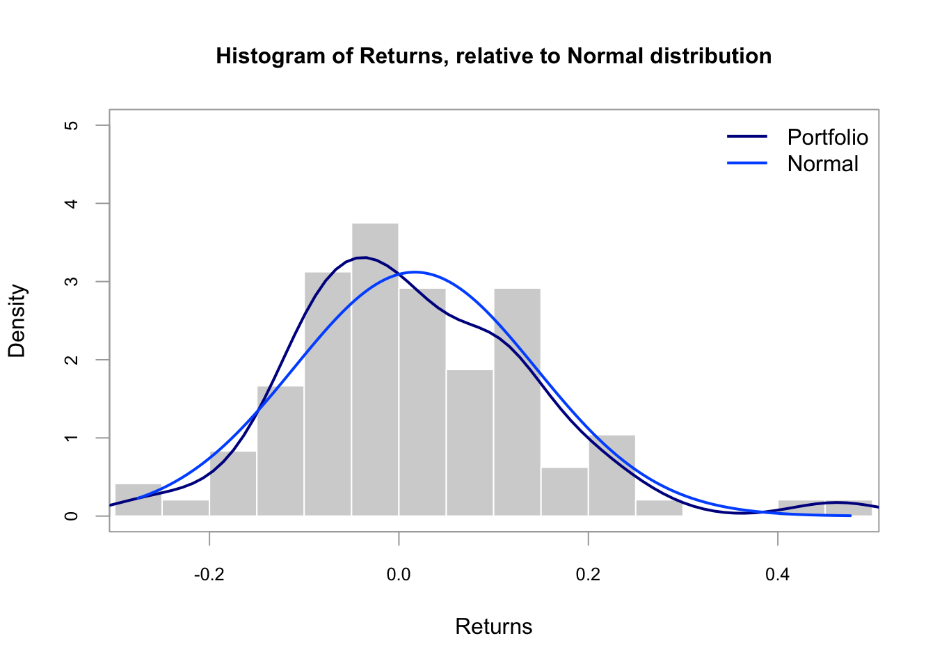
Skewness and Kurtosis
Skewness
\(\mu_3\) is the third (normalized) moment about the mean.
It measures the asymmetry of the distribution, with symmetric distribution having \(\mu_3=0\).
- \(\mu_3>0\) means positively skewed, i.e., long right tail.
- \(\mu_3<0\) means negatively skewed, i.e., long left tail.
\[ \mu_3 = \frac{1}{T} \frac{\sum_{t=1}^T (r_{p,t}-\bar{r}_p)^3}{\sigma_p^3} \]
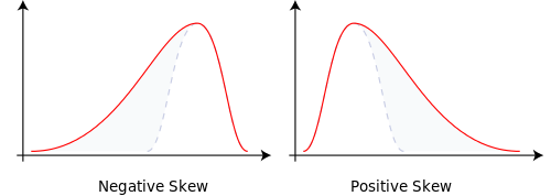
Fig. 5: Diagram of Skewness.
# skewness
skewness(ptf_xts$port_ret)
## port_ret
## 0.7779903Kurtosis
\(K_p\) is the fourth (normalized) moment about the mean.
It measures the tail behavior in comparison with the normal distribution.
\[ \mu_4 = \frac{1}{T} \frac{\sum_{t=1}^T (r_{p,t}-\bar{r}_p)^4}{\sigma_p^4} \]
The kurtosis for any normal distribution is three. For this reason, we subtract three from \(\mu_4\) to get the “excess kurtosis”.
- \(\mu_4-3>0\) indicate a heavy-tailed distribution with higher chances of outliers.
- \(\mu_4-3<0\) indicate a light-tailed distribution with lower chances of outliers.
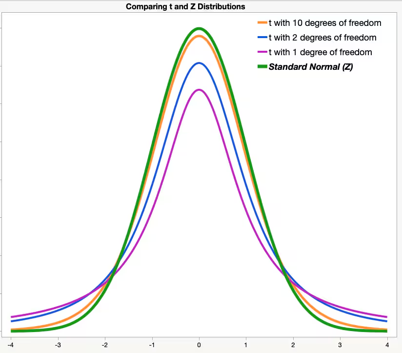
Fig. 6: Examples of heavy-tailed distributions.
\(t\)-distribution has higher kurtosis than normal distributions.
- Meaning that \(t\)-distribution has a higher probability of obtaining values that are far from the mean than a normal distribution.
- It is less peaked in the center and higher in the tails than normal distribution.
- As the degree of freedom increases, \(t\)-distribution approximates to normal distribution, kurtosis decreases and approximates to 3.
set.seed(125)
rnorm(1000) %>% moments::kurtosis()
## [1] 3.037806rt(1000, df=1) %>% moments::kurtosis()## [1] 503.3928rt(1000, df=2) %>% moments::kurtosis()## [1] 61.25994rt(1000, df=10) %>% moments::kurtosis()## [1] 4.303517rt(1000, df=30) %>% moments::kurtosis()## [1] 3.646411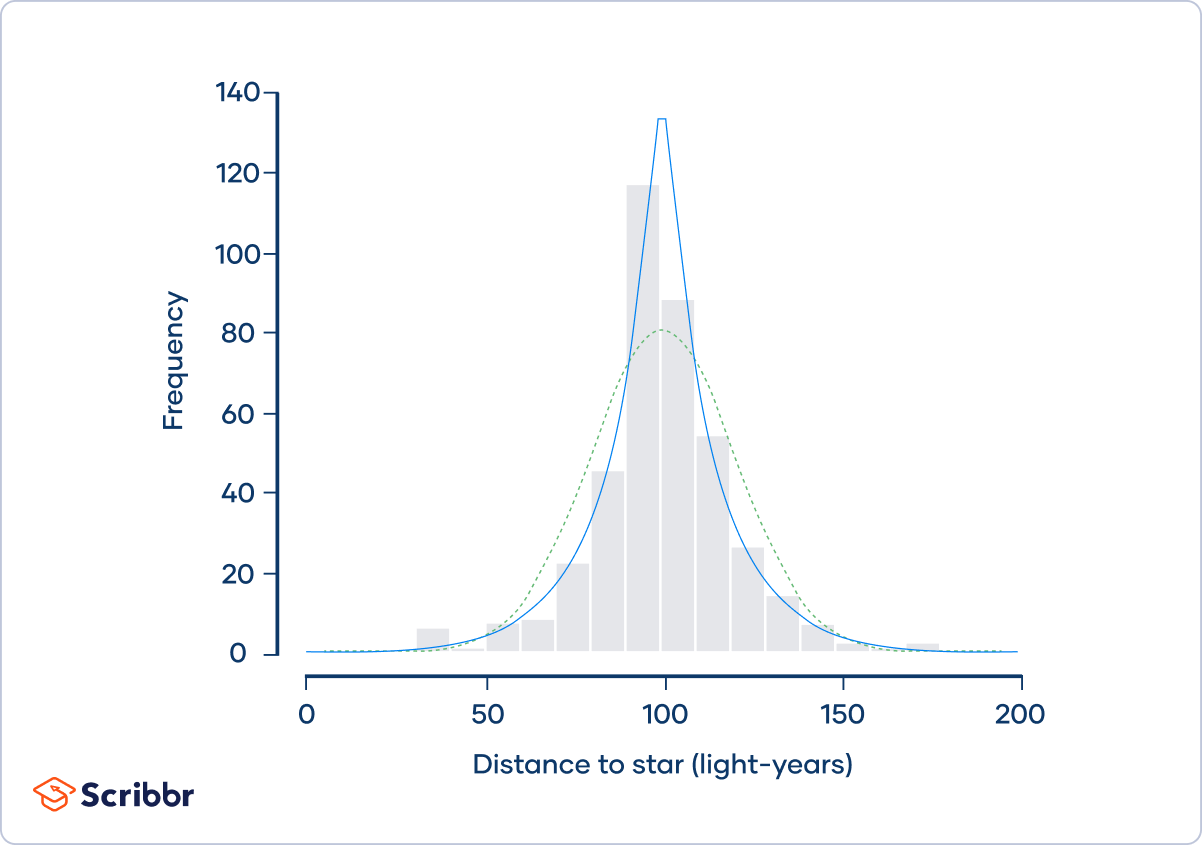
Fig. 7: Laplace distribution. The dotted green curve shows a normal distribution. The blue curve shows a Laplace distribution with kurtosis of 6.54. On the far left and right sides of the distribution—the tails—the space below the Laplace distribution curve (blue) is slightly thicker than the space below the normal distribution curve (green). This is an example of a heavy-tailed distribution yet with a sharper peak.
Distinguish from standard deviation/variance.
Standard deviation and kurtosis are both measures of the variability of a distribution, but they are not directly related.
Two distributions with identical means and standard deviations can have very different shapes, and kurtosis is one of the measures of that difference.
It looks at how much of the ‘weight’ of the distribution (recall that the total weight, or the area under the curve, is 1) is sitting in the tails as opposed to the middle of the distribution.
- Standard deviation is useful for measuring the spread.
- Kurtosis focuses on detecting outliers.
PerformanceAnalytics::kurtosis(x, na.rm = FALSE, method = "excess") returns excess kurtosis by default.
Need to specify method = "moment" in order to get the original kurtosis.
moments::kurtosis(x) returns the original kurtosis. Need to be compared with 3 on your own.
# kurtosis
moments::kurtosis(ptf_xts$port_ret)
## port_ret
## 4.69699PerformanceAnalytics::kurtosis(ptf_xts$port_ret) # excess kurtosis## [1] 1.69699PerformanceAnalytics::kurtosis(ptf_xts$port_ret, method = "moment") # original kurtosis## [1] 4.69699PerformanceAnalytics::table.Stats(R, ci = 0.95, digits = 4) returns a full set of summary statistics that match the period of the data passed in (e.g., monthly returns will get monthly statistics, daily will be daily stats, and so on)
# summary statistic
returns_statistics <- table.Stats(ptf_xts$port_ret)
returns_statistics %>%
    knitr::kable() %>%
    kable_styling(bootstrap_options = c("striped", "hover"),
full_width = F, latex_options="scale_down") | port_ret | |
|---|---|
| Observations | 96.0000 |
| NAs | 0.0000 |
| Minimum | -0.2754 |
| Quartile 1 | -0.0680 |
| Median | 0.0014 |
| Arithmetic Mean | 0.0168 |
| Geometric Mean | 0.0092 |
| Quartile 3 | 0.1008 |
| Maximum | 0.4766 |
| SE Mean | 0.0131 |
| LCL Mean (0.95) | -0.0091 |
| UCL Mean (0.95) | 0.0427 |
| Variance | 0.0164 |
| Stdev | 0.1279 |
| Skewness | 0.7780 |
| Kurtosis | 1.6970 |
SE Mean: Standard Error of the average return.\[ \text{SE Mean} = \frac{\sigma_p}{\sqrt{T}} \]
LCL Mean: Lower Confidence Level (LCL) of the mean, defaults to 95% confidence level.\[ \text{LCL Mean} = \bar{r}_p - \text{SE Mean} \times c_{\alpha/2} \]
where \(c_{\alpha/2}\) is the critical value, i.e., \(\left(1-\frac{\alpha}{2}\right)\) quantile of the \(t\) distribution with \((T-1)\) degrees of freedom.
UCL Mean: Upper Confidence Level (UCL) of the mean, defaults to 95% confidence level.\[ \text{UCL Mean} = \bar{r}_p + \text{SE Mean} \times c_{\alpha/2} \]
Kurtosis: Excess Kurtosis.
Information ratio
While the Sharpe ratio measures the excess return as the difference between the return of the portfolio and the risk-free rate, the information ratio, on the other hand, measures the portfolio performance against a comparable benchmark rather than the risk-free rate.
The information ratio is the active return per unit of active risk. This relates the degree to which an investment has beaten the benchmark to the consistency with which the investment has beaten the benchmark.
\[ \begin{aligned} \text{Information Ratio} &= \text{IR}_p = \frac{\bar{r}_p-\bar{r}_m}{\sigma_{p-m}} \\ \text{Annualized Informatione Ratio} &= \text{IR}_p^A = \frac{\bar{r}_p-\bar{r}_m}{\sigma_{p-m}} \times \sqrt{12} \end{aligned} \] where
- \(\bar{r}_p\) and \(\bar{r}_m\) is the average return for the portfolio and the benchmark, respectively;
- \(\bar{r}_p-\bar{r}_m\) is the active return (or active premium) of the portfolio, i.e., return of portfolio in excess of the benchmark return;
- \(\sigma_{p-m}\) is the active risk (or tracking error) of the portfolio, i.e., the standard deviation (volatility) of the active return.
Beta coefficient-adjusted measures
Sharpe and Information ratios use standard deviation as the measure of portfolio risk. An alternative risk measure is the beta coefficient based on the CAPM model.
Recall that the beta coefficient can be estimated using the follow regression
\[ r_{i,\color{red}{t}} - r_{f,\color{red}{t}} = \alpha_i + \beta_i (r_{m,\color{red}{t}}-r_{f,\color{red}{t}}) + \varepsilon_{i,\color{red}{t}} . \] The OLS \(\beta_i\) estimate can be expressed as
\[ \hat{\beta}_i = \frac{\text{Cov}(R_{m}^e, R_{i}^e)}{\text{Var}(R_{i}^e)} \] where
- \(R^e_i=r_i-r_f\) stands for the excess return on asset \(i\), and
- \(R^e_m=r_m-r_f\) stands for the excess return on the market index.
Treynor ratio is a variant of Sharpe ratio. It substitute the standard deviation in Sharpe ratio with the beta coefficient.
The Treynor ratio is computed as
\[ \text{Treynor Ratio}_p = \frac{\bar{r}_p-\bar{r}_f}{\beta_p} \] Note that
the only relevant risk in the computation of the Treynor ratio is systematic risk. It assumes that the portfolio is fully diversified. Appropriate for diversified equity funds, the element of unsystematic risk would be negligible.
Sharpe ratio assumes that the relevant risk is total risk (systematic and unsystematic risk), and it measures excess return per unit of total risk. It is appropriate for the portfolio that is less diversified.
Jensen’s alpha also assumes that the relevant risk is systematic risk.
Jensen’s alpha measures the average return on the portfolio in excess of what predicted by the CAPM, given the portfilio’s beta and the average market return.
\[ \alpha_p = \bar{r}_p - \left[\bar{r}_f + \beta_p(\bar{r}_m-\bar{r}_f)\right] \]
Exercise
Given the following information about the return on a portfolio, the market index and risk free returns.
| Year | Portfolio | Market index | Risk free rate |
| 1 | 14% | 12% | 7% |
| 2 | 10 | 7 | 7.5 |
| 3 | 19 | 20 | 7.7 |
| 4 | -8 | -2 | 7.5 |
| 5 | 23 | 12 | 8.5 |
| 6 | 28 | 23 | 8 |
| 7 | 20 | 17 | 7.3 |
| 8 | 14 | 20 | 7 |
| 9 | -9 | -5 | 7.5 |
| 10 | 19 | 16 | 8 |
| Average | 13% | 12% | 7.6% |
| Standard deviation | 12.39% | 9.43% | 0.47% |
| Cov(\(r_p\), \(r_m\)) | 0.0107 |
- Calculate the beta.
\[ \beta_p = \frac{\text{Cov}(r_p, r_m)}{\text{Var}(r_m)} = \frac{0.0107}{9.43\%^2} = 1.203 \]
- Calculate the Sharpe ratio.
\[ S_p = \frac{\bar{r}_p-\bar{r}_f}{\sigma_p} = \frac{(13-7.6)\%}{12.39\%} = 0.436 \]
- Calculate the Treynor ratio.
\[ T_p = \frac{\bar{r}_p-\bar{r}_f}{\beta_p} = \frac{(13-7.6)\%}{1.203} = 0.0449 \]
- Calculate Jensen’s Alpha.
\[ \alpha_p = \bar{r}_p - \left[\bar{r}_f + \beta_p(\bar{r}_m-\bar{r}_f)\right] = 13\% - 7.6\% - 1.203\times (12-7.6)\% = 0.107\% \]
M-squared
The M-squared (\(M^2\)) measure is first introduced by Franco Modigliani. \(M^2\) provides a direct comparison between the leverage-adjusted portfolio and the market portfolio.
A managed portfolio \(p\) is mixed with a position in the risk free asset to make the “leverage-adjusted” (or “adjusted” in short) portfolio have the same volatility as the market. Suppose the managed portfolio p has a total variability equal to \(1.5\times \sigma_m\). The “adjusted” portfolio \(p^*\) is found by investing a weight \(w\) in \(p\) and a weight \((1 − w)\) in the risk free asset, such that the portfolio has the same standard deviation as the market:
\[ \begin{aligned} r_{p^*} &= w\, r_p + (1-w)\, r_f \\ \sigma_{p^*} &= w\sigma_p + (1-w)\sigma_{r_f} = w\sigma_p + (1-w)\cdot 0 = w\sigma_p \end{aligned} \] Let
\[ \sigma_{p^*} = \sigma_m , \] we have
\[ w\sigma_p = \sigma_m \Rightarrow w=\frac{\sigma_m}{\sigma_p} = \frac{\sigma_m}{1.5\sigma_m} = \frac{2}{3} \] By investing two thirds in \(p\) and one third in the risk free asset \(r_f\), achieve the same volatility as the market.
Since \(P^∗\) and \(m\) have the same volatility, we may compare their returns simply by calculating the difference:
\[ M_p^2 = r_{p^*} - r_m . \]
Downside risk measures
When the return distribution is asymmetric (skewed), investors use additional risk measures that focus on describing the potential losses.
The Semi-Deviation is the calculation of the variability of returns below the mean return. \[ \begin{aligned} \text{Semi } \sigma_p &= \sqrt{\frac{1}{n}\textstyle \sum_{t=1}^T \big[\min(r_{p,t}-\bar{r}_p, 0)\big]^2 } \\ \text{Annualized Semi } \sigma_p^A &= \sqrt{\frac{1}{n}\textstyle \sum_{t=1}^T \big[\min(r_{p,t}-\bar{r}_p, 0)\big]^2 } \times \sqrt{12} \end{aligned} \] where \(n\) is either the number of observations of the entire series or the number of observations in the subset of the series falling below the average.
Value-at-Risk (VaR) measures the potential loss in value of a risky asset or portfolio over a defined period for a given confidence interval. It corresponds to a probability \(p\), which is a confidence level.
A \(p\) VaR means that the probability of a loss greater than VaR is (at most) \((p)\) while the probability of a loss less than VaR is (at least) \(1-p\).
For example, a one-day \(5\%\) VaR of \(\$1\) million implies the portfolio has a \(5\%\) chance that the value of the asset drops more than \(\$1\) million over one day. In other words, there is a \(95\%\) probability that the asset makes a profit or lose less than \(\$1\) million over a day.
Different conventions are used for \(p\). You can tell by the magnitude whether it refers to a confidence level or a significance level. For instance, sometimes you see \(95\%\) VaR (confidence level) and \(5\%\) VaR (significance level).
To obtain a sample estimate of \(5\%\) VaR, we sort the observations from high to low. The VaR is the return at the \(5\)th percentile of the empirical sample distribution.
More formally, \[ \text{VaR}(\alpha) = -F^{-1}(\alpha) \] where \(F(\cdot)\) is the cdf of the portfolio return \(r_p\).
The expected shortfall (ES) is the expected value of the loss, given the loss is greater than the VaR.
\[ \text{ES}(\alpha) = E[r_p \vert r_p \leq F^{-1}(\alpha)] \]
- VaR is the most optimistic measure of worst-case scenarios as it takes the smallest loss of all these cases, while ES informs the magnitudes of potential losses given that the loss is greater than the VaR.
## downside risk measures
# Calculate the SemiDeviation
SemiDeviation(ptf_xts$port_ret)
## port_ret
## Semi-Deviation 0.08114918sd(ptf_xts$port_ret)## [1] 0.1278693# Calculate the value at risk, p is the confidence level
VaR(ptf_xts$port_ret, p=.95) # 95% VaR## port_ret
## VaR -0.1584788VaR(ptf_xts$port_ret, p=.99) # 99% VaR## port_ret
## VaR -0.2278215# Calculate the expected shortfall
ES(ptf_xts$port_ret, p=.95)## port_ret
## ES -0.1913056ES(ptf_xts$port_ret, p=.99)## port_ret
## ES -0.2278215The other popular downside risk estimate, the maximum drawdown (MDD) of the portfolio, measures the largest loss from peak to trough over the examination period.
The maximum drawdown of the portfolio indicates the maximum possible loss investors have ever experienced over the examination period.
\[ MDD = \frac{LP-PV}{PV} \]
- where \(LP\) is the lowest value after peak value, this is also called “Trough Value”;
- \(PV\) is the peak value.
# Table of drawdowns
maxDrawdown(ptf_xts$port_ret)
## [1] 0.5840139table.Drawdowns(ptf_xts$port_ret)## From Trough To Depth Length To Trough Recovery
## 1 2018-06-30 2020-03-31 2021-03-31 -0.5840 34 22 12
## 2 2015-06-30 2016-02-29 2016-12-31 -0.5637 19 9 10
## 3 2022-02-28 2022-04-30 2022-12-31 -0.2388 11 3 8
## 4 2017-08-31 2017-11-30 2018-05-31 -0.2232 10 4 6
## 5 2015-01-31 2015-02-28 2015-04-30 -0.1607 4 2 2# Plot of drawdowns
chart.Drawdown(ptf_xts$port_ret)
Rolling performance
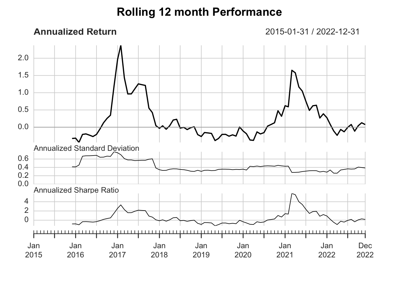
Rolling performance is typically used as a way to assess stability of a return stream.
A rolling window of 12 months is NOT the same as annually.
Rolling window of 12 mons: The window “rolls” forward one month at a time. The data frequency is monthly.
For example, it computes return from Jan–Dec 2015, then Feb 2015–Jan 2016, then Mar 2015–Feb 2016, and so on. This gives you a smoother, more continuous view of how performance evolves over time.
Annual performance calculates returns or metrics strictly once per calendar year (e.g., Jan–Dec 2015, Jan–Dec 2016). The data frequency is annually.
Each year is treated as a discrete block. There’s no overlap between years.
Key differences:
| Aspect | Rolling 12-Month Window | Annual (Calendar Year) |
|---|---|---|
| Frequency | Monthly | Yearly |
| Overlapping Periods | Yes | No |
| Smoothness | Smoother trends | Step-wise, discrete jumps |
| Use Case | Trend analysis, risk over time | Year-by-year comparison |
| Number of Observations | Higher | Lower |
PerformanceAnalytics::chart.RollingPerformance(R, width = 12, FUN = "Return.annualized") provides a way to display different metrics, e.g., returns, standard deviation, Sharpe ratio, over rolling time periods.
width: number of periods to apply rolling function window over.FUN: any function that can be evaluated using a single set of returns.
## rolling annualized mean
chart.RollingPerformance(R = ptf_xts$port_ret, width = 12, FUN = "Return.annualized")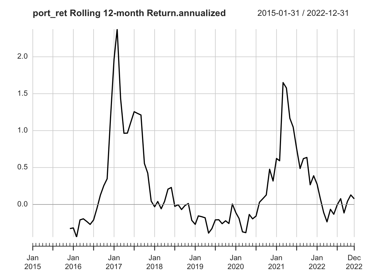
## rolling annualized volatility
chart.RollingPerformance(R = ptf_xts$port_ret, width = 12, FUN = "StdDev.annualized")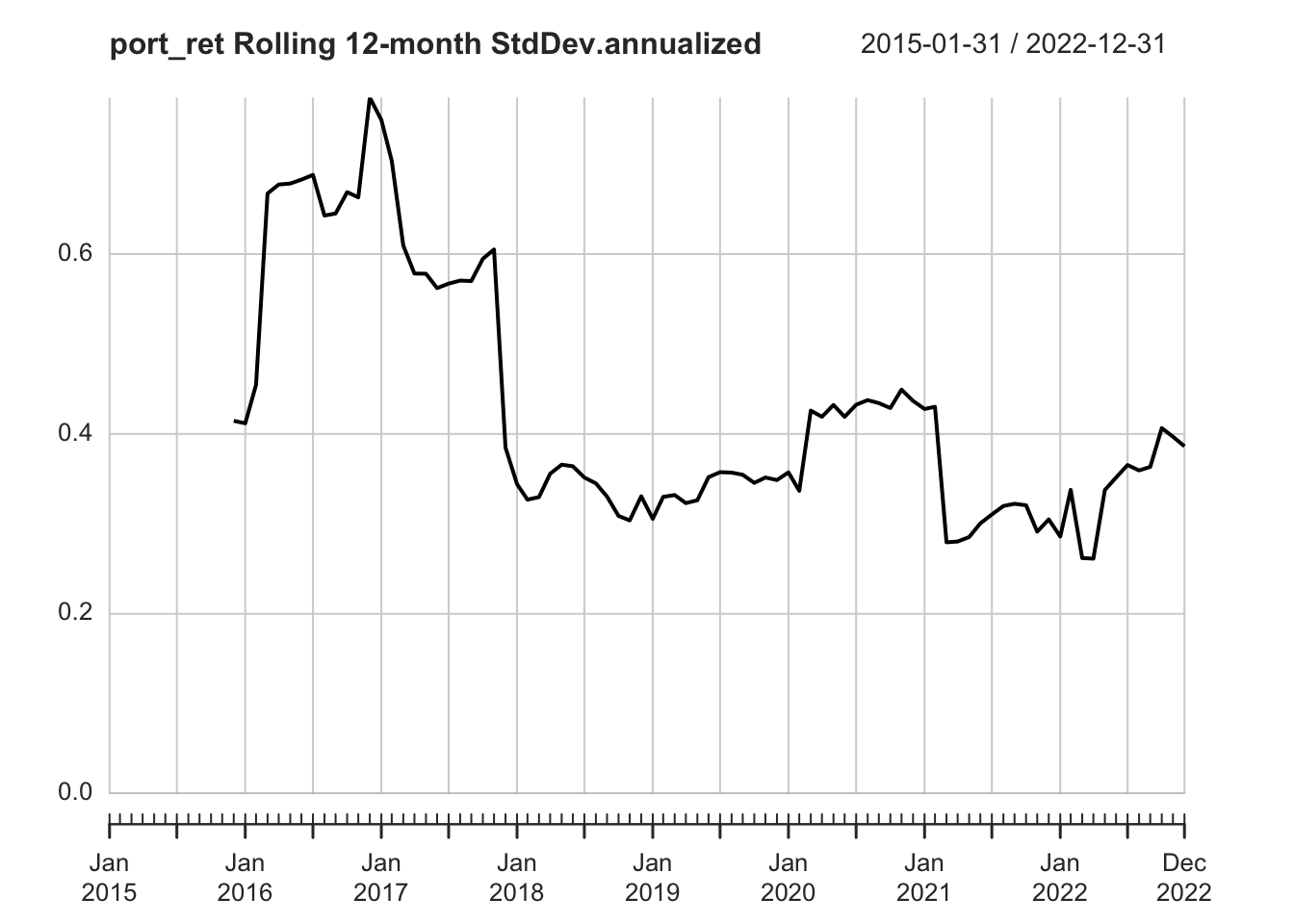
## rolling annualized Sharpe ratio
chart.RollingPerformance(R = ptf_xts$port_ret, width = 12, FUN = "SharpeRatio.annualized", Rf=ptf_xts$rf_1month)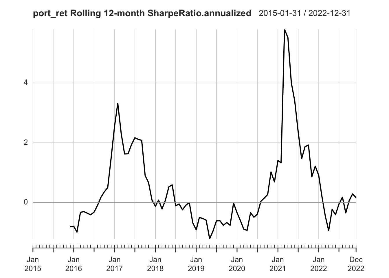
Three-in-one rolling performance charts can be created using charts.RollingPerformance.
charts.RollingPerformance(R = ptf_xts$port_ret, width = 12, Rf=ptf_xts$rf_1month)