Probability and Data in Business Analytics
Probability is the foundation for making data-driven decisions in business. This section covers the essential concepts, formulas, and business examples you’ll use in analytics.
1 Probability Axioms
Probability measures how likely an event is.
\[P(A) = \frac{\text{Number of ways A can occur}}{\text{Total possible outcomes}}\]
- \(P(A) \geq 0\) for any event \(A\)
- \(P(\text{all possible outcomes}) = 1\)
- \(P(A \text{ or } B) = P(A) + P(B) - P(A\text{ and }B)\)
- If \(A\) and \(B\) are mutually exclusive, then \[ P(A \text{ and } B) = 0 \] and \[ P(A \text{ or } B) = P(A) + P(B) \] Mutually exclusive means “cannot happen together.”
Example 1 A retailer estimates a 30% chance of a supply chain disruption and a 50% chance of a demand spike. If these events are mutually exclusive, what is the probability of either event occurring?
Solution 1. Since the events are mutually exclusive, \(P(A \text{ and } B)=0,\) then \[ \begin{split} P(A \text{ and } B)=P(A)+P(B)-P(A \text{ and } B)=0.30+0.50=0.80. \end{split} \]
Example 2 In a multi-channel marketing campaign, 35% of customers click an email offer (Event A) and 25% engage with a social media ad (Event B). Data shows 10% of customers do both. What is the probability a randomly selected customer engages with at least one of the two channels (email OR social)?
Solution 2.
\(P(A) + P(B) - P(A \text{ and } B) = 0.35 + 0.25 - 0.10 = 0.50\)2 Sample vs. Population: Estimating the Big Picture
In business, we use samples to estimate population characteristics.
Sample mean:
\[ \overline{X} = \frac{1}{n} \sum_{i=1}^n X_i \]
Example 3 A telecom company surveys a randomly selected sample of 500 customers about service quality. The sample mean satisfaction score is 4.2. How can this estimate help guide company-wide improvements?
Solution 3.
- The sample mean (4.2) is based on 500 surveyed customers (the sample).
- The population is all customers of the telecom company.
- To guide company-wide improvements, we need to know if the sample is representative of the population.
- There is uncertainty in the estimate; larger samples make the sample mean closer to the true population mean.
- The sample mean is useful, but its reliability depends on sample representativeness and size.
Example 4 Why is it important to distinguish between sample and population in business analytics?
Solution 4.
Because we use samples to estimate population parameters, and understanding the difference helps us make better decisions and avoid bias.3 Moments
3.1 Expectation, Variance, and Standard Deviation
Expectation (population): Average level of the outcome (true but unknown in practice). \[ \mathbb{E}[X] = \begin{cases} \displaystyle \sum_{i} x_i \, P(X = x_i) & \text{(discrete)} \\ \displaystyle \int_{-\infty}^{\infty} x \, f(x) \, dx & \text{(continuous)} \\ \end{cases} \] Sample estimator: Replace the distribution by observed data: \[\bar{X} = \dfrac{1}{n}\sum_{i=1}^n X_i.\] The sample mean \(\bar{X}\) estimates the population mean \(\mathbb{E}[X]\).
Variance (population): How much values fluctuate around the true mean.
\[\text{Var}(X) = E[(X - E[X])^2]\]
The variance can also be expressed as:
\[ \begin{aligned} \color{#00CC66}{\text{Var}(X)} &= \mathbb{E}\left[\left(X - \mathbb{E}[X]\right)^2\right] \\ &= \color{#00CC66}{\mathbb{E}[X^2] - (\mathbb{E}[X])^2}. \end{aligned} \]
This second form is often faster to compute when you already have (or can easily get) \(\mathbb{E}[X^2]\) (e.g., from grouped data or a probability model). In finance, we frequently estimate variance from simulated or historical returns by computing the average of squared returns (giving \(\mathbb{E}[X^2]\)) and subtracting the square of the average return.
Sample estimators:
- Biased (population style) estimator: \[ \hat{\sigma}^2 = \dfrac{1}{n}\sum_{i=1}^n (X_i - \bar{X})^2 \]
- Unbiased estimator: \[s^2 = \dfrac{1}{n-1}\sum_{i=1}^n (X_i - \bar{X})^2 \] The latter (\(s^2\)) subtracts 1 from \(n\) in the denominator, which is known as a degrees of freedom correction. This version has some desirable properties but we will not discuss these for now. Suffice to say that both versions are usually fine.
Example 5 An operations planner models next-hour demand arrivals for a micro-warehouse (number of urgent orders) as \(X \in \{0,1,2\}\) with probabilities 0.2, 0.5, 0.3. Compute the variability (variance) of order arrivals using the shortcut formula \(\mathbb{E}[X^2] - (\mathbb{E}[X])^2\) to inform staffing.
Solution 5. \[ \begin{split} \mathbb{E}[X] &= 0(0.2)+1(0.5)+2(0.3)=1.1 \\ \mathbb{E}[X^2] &= 0^2(0.2)+1^2(0.5)+2^2(0.3)=0+0.5+1.2=1.7 \\ \text{Var}(X) &= \mathbb{E}[X^2] - (\mathbb{E}[X])^2 = 1.7 - 1.1^2 = 1.7 - 1.21 = 0.49 \end{split} \]
Example 6 A SaaS company tracks daily change in Daily Active Users (DAU) (in %) over 5 days: \(0.4\), \(0.6\), \(-0.2\), \(0.5\), \(0.7\). Verify that the direct variance definition and the shortcut formula match; interpret what the variance implies for short‑term engagement volatility.
Solution 6. Daily % changes: \(0.4,\ 0.6,\ -0.2,\ 0.5,\ 0.7\). Let units be percentage points (pp). \[
\mathbb{E}[X] = \frac{0.4+0.6-0.2+0.5+0.7}{5} = 0.4 \text{ pp}
\] \[
\mathbb{E}[X^2] = \frac{0.16+0.36+0.04+0.25+0.49}{5} = \frac{1.30}{5} = 0.26 \text{ (pp)}^2
\] Variance (percentage-point squared): \[
\text{Var}(X) = 0.26 - (0.4)^2 = 0.26 - 0.16 = 0.10 \text{ (pp)}^2
\] Standard deviation \(= \sqrt{0.10} \approx 0.316\) pp (about \(0.32\) percentage points). Direct (long) method matches (0.10).
Interpretation: Moderate short-term volatility compared to the mean change of 0.4 pp. This suggests some fluctuations in user engagement, but not extreme.
Standard Deviation (population): Square root of variance, showing average deviation from the true mean.
\[\text{sd}(X) = \sqrt{\text{Var}(X)}\]
Sample estimator: \(s = \sqrt{s^2}\) (using the unbiased \(s^2\) above).
Example 7 A hedge fund analyzes daily returns of two portfolios. Portfolio A has higher mean but also higher variance. How should risk-adjusted performance be compared?
Solution 7.
Compare risk-adjusted metrics (e.g., Sharpe ratio = (mean - rf)/sd). Higher mean with disproportionate variance may yield lower Sharpe.Example 8 A business has daily profits of $200, $250, $180, $220, and $210. Calculate the mean and variance.
Solution 8. Mean: \(\bar{x}=\dfrac{200+250+180+220+210}{5}=\dfrac{1060}{5}=212\).
Variance calculations:
- Sum of squared deviations
\[ \begin{aligned} (200-212)^2 &+ (250-212)^2 + (180-212)^2 + (220-212)^2 + (210-212)^2 \\ &= 144 + 1444 + 1024 + 64 + 4 = 2680 \end{aligned} \] - Population variance (divide by \(n=5\))
\[ \sigma^2 = \frac{2680}{5} = 536 \] - Sample variance (unbiased, divide by \(n-1=4\))
\[ s^2 = \frac{2680}{4} = 670 \]
Population variance uses \(n\) when treating these 5 observations as the entire population; sample variance uses \(n-1\) to unbiasedly estimate \(\text{Var}(X)\) of a larger process.
3.2 Sums of Random Variables: Expectation & Variance
Population linearity of expectation: \[E[X + Y] = E[X] + E[Y]\]
Sample counterpart: \(\overline{X+Y} = \bar{X} + \bar{Y}\) (sample means add componentwise).
If \(X\) and \(Y\) are independent, the population variance of their sum is the sum of their variances: \[\text{Var}(X + Y) = \text{Var}(X) + \text{Var}(Y)\]
If not independent, add twice the covariance: \[\text{Var}(X + Y) = \text{Var}(X) + \text{Var}(Y) + 2\text{Cov}(X, Y)\]
Sample counterpart (unbiased style): \[s_{X+Y}^2 = s_X^2 + s_Y^2 + 2 s_{XY},\] where \(s_{XY} = \dfrac{1}{n-1}\sum_{i=1}^n (X_i-\bar{X})(Y_i-\bar{Y}).\)
Intuitive Example: In portfolio management, the total risk (variance) of a portfolio depends on the variances of individual assets and how they move together (covariance).
Example 9 Two independent projects have profit variances of 100 and 150. What is the variance of total profit?
Solution 9.
\(100 + 150 = 250\).Variance of Linear Transformations & Portfolios
The variance operator is the expectation of a quadratic function, so it is not linear. Instead, for constants \(a, b\):
\[ \text{Var}(a + bX) = b^2\,\text{Var}(X). \]
More generally, for constants \(a_i \in \mathbb{R}, i=1,\ldots,n\):
\[ \text{Var}\left(\sum_{i=1}^n a_i X_i \right) = \sum_{i=1}^n a_i^2 \, \text{Var}(X_i) + \sum_{i=1}^n \sum_{j=1}^n a_i a_j \, \text{Cov}(X_i, X_j). \]
If the \(X_i\) are pairwise independent (or uncorrelated), the double sum of covariance terms drops out for \(i\neq j\), leaving only the first sum.
Example 10 A portfolio allocates 40% to Asset A and 60% to Asset B. \(\text{Var}(A)=0.04\), \(\text{Var}(B)=0.09\), and \(\text{Cov}(A,B)=0.01\). Compute portfolio variance using the general formula.
Solution 10.
\(\text{Var}(P)=0.4^2(0.04)+0.6^2(0.09)+2(0.4)(0.6)(0.01)=0.0064+0.0324+0.0048=0.0436\).Example 11 A production planner combines forecasts: Final forecast \(F = 2 + 0.7X_1 + 0.3X_2\). If \(\text{Var}(X_1)=25\), \(\text{Var}(X_2)=9\), and \(\text{Cov}(X_1,X_2)=6\), find \(\text{Var}(F)\).
Solution 11.
Constant 2 adds no variance. \(\text{Var}(F)=0.7^2(25)+0.3^2(9)+2(0.7)(0.3)(6)=12.25+0.81+2.52=15.58\).3.3 Skewness
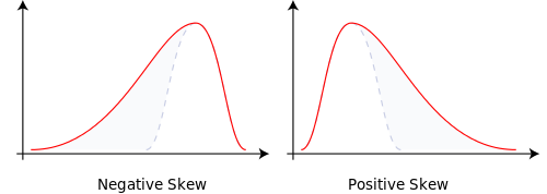
Skewness measures asymmetry in a distribution.
- Skewness = 0: Symmetric (e.g., normal)
- Skewness < 0: Longer left tail (large losses more likely than large gains)
- Skewness > 0: Longer right tail (occasional big gains)
Business reading: Positive skew in quarterly sales means you usually hit average numbers but sometimes land a very big contract. Negative skew in operational losses could mean rare but severe downside events that need contingency planning.
Let \(\mu_3 = E[(X-\mathbb{E}[X])^3]\) denote the third central moment. Standardized (population) skewness: \[\gamma_1 = \frac{\mu_3}{\text{sd}(X)^3}.\]
Sample (bias‑adjusted) skewness estimator: \[\hat{\gamma}_1 = \frac{n}{(n-1)(n-2)} \sum_{i=1}^n \left(\frac{X_i-\bar{X}}{s}\right)^3.\]
Tip
Note for skewness and kurtosis, it is NOT expected to hand calculate the values, the focus is on
- the interpretation of given results.
- be able to recognize skewness and kurtosis in data visualizations (e.g., histograms, box plots).
3.4 Kurtosis
Kurtosis measures tail weight (propensity for outliers) relative to a normal distribution.
- Kurtosis ≈ 3: Normal tail thickness
- Kurtosis > 3 (leptokurtic): Heavy / fat tails, more extreme outcomes
- Kurtosis < 3 (platykurtic): Light / thin tails, fewer extremes

\(t\)-distribution has higher kurtosis than normal distributions.
- Meaning that \(t\)-distribution has a higher probability of obtaining values that are far from the mean than a normal distribution.
- It is less peaked in the center and higher in the tails than normal distribution.
- As the degree of freedom increases, \(t\)-distribution approximates to normal distribution, kurtosis decreases and approximates to 3.
For the \(t\)-distribution:
- As the degrees of freedom (df) increase, the \(t\)-distribution approaches the normal distribution.
- A common rule of thumb is that for \(df > 30\), one can pretty safely use the normal distribution in place of a t-distribution unless you are interested in the extreme tails.
Let \(\mu_4 = E[(X-\mathbb{E}[X])^4]\) be the fourth central moment. Standardized (population) kurtosis: \[\kappa = \frac{\mu_4}{\text{sd}(X)^4}, \qquad \text{Excess kurtosis} = \kappa - 3.\] Sample (Fisher) excess kurtosis estimator: \[\hat{g}_2 = \frac{n(n+1)}{(n-1)(n-2)(n-3)} \sum_{i=1}^n \left(\frac{X_i-\bar{X}}{s}\right)^4 - \frac{3(n-1)^2}{(n-2)(n-3)}.\] High excess kurtosis signals greater tail risk; low or negative excess indicates fewer extreme outcomes.
Interpretation link: High positive skewness without high kurtosis means upside spikes with limited extra tail risk; high kurtosis (regardless of skew sign) means fatter tails and a need to focus on outlier management.
Example 12 A company’s quarterly profits have excess kurtosis of 4. What does this mean for risk management?
Solution 12. Excess kurtosis is defined relative to a normal distribution (which has kurtosis 3).
- Excess kurtosis = Kurtosis − 3
- So an excess kurtosis of 4 means the total kurtosis is 7, much higher than a normal distribution.
This implies the distribution of quarterly profits has fat tails — extreme profit or loss outcomes are more likely than under a normal distribution. Recommend to focus risk management on outliers.
4 Covariance, Correlation & Independence
Population covariance measures the direction of comovement between two variables:
- Positive covariance: Both variables increase or decrease together
- Negative covariance: One increases while the other decreases
- Magnitude: Does not indicate strength of relationship
Population formulas: \[\text{Cov}(X, Y) = E[(X - E[X])(Y - E[Y])]\] \[\text{Cov}(X, Y) = E[XY] - E[X]E[Y]\]
Sample covariance (unbiased): \[s_{XY} = \frac{1}{n-1}\sum_{i=1}^n (X_i - \bar{X})(Y_i - \bar{Y}).\]
Population correlation standardizes covariance to a scale from -1 to 1: \[\text{Corr}(X, Y) = \frac{\text{Cov}(X, Y)}{\text{sd}(X) \cdot \text{sd}(Y)}\]
Sample correlation: \[r_{XY} = \frac{s_{XY}}{s_X s_Y}.\]
- Correlation = 1: Perfect positive relationship
- Correlation = \(-1\): Perfect negative relationship
- Correlation = 0: No linear relationship
Independence means knowing one event doesn’t affect the other: \[P(A \text{ and } B) = P(A) \cdot P(B)\]
Independence vs. Correlation
Independence means no influence between events, while correlation measures linear relationship strength.
Independence implies zero correlation, but zero correlation does not imply independence.
E.g., \(X\) and \(Y = X^2\) have zero correlation but are not independent.
Business Example: Suppose a retailer finds that sales and weather are correlated. This information can be used to adjust inventory planning for seasonal effects. If two marketing campaigns are independent, the outcome of one does not affect the other.
Example 13 Suppose a customer visits a supermarket. Let:
- \(A\) = “customer buys a loaf of bread today” and \(P(A)=30\%\).
- \(B\) = “customer buys laundry detergent today” and \(P(B)=10\%\).
What is the probability the customer buys both bread and detergent today? What does observing a bread purchase tell you about \(P(B)\)?
Solution 13. Bread (frequent staple) and detergent (infrequent refill) decisions are unrelated, so it is reasonable to assume independence. Hence \[ P(A \text{ and } B) = 30\% \times 10\% = 3\% \] Observing bread does not change \(P(B)=10\%\).
Example 14 If the correlation between two stocks is \(-0.8,\) what does this mean for portfolio diversification?
Solution 14.
They tend to move in opposite directions, aiding diversification and reducing portfolio variance.
Mutually Exclusive vs Independence
Mutually exclusive: Cannot happen together \[P(A\cap B)=0\]
Independent: Knowledge of one does not change probability of the other \[P(A\cap B)=P(A)P(B)\]
Think: Disjoint = “never together”; Independent = “no influence”.
5 Population vs. Sample: Summary & Estimators
When analysing data we distinguish between:
- Population parameters (target): Fixed (but usually unknown) numerical characteristics of the underlying process (e.g., \(\mathbb{E}[X], \text{Var}(X), \gamma_1, \kappa, \text{Cov}(X,Y)\)).
- Sample statistics (estimators): Functions of observed data used to approximate population parameters (e.g., \(\bar{X}, s^2, s, \hat{\gamma}_1, \hat{g}_2, s_{XY}, r_{XY}\)). They vary from sample to sample.
Key principles:
- Replace integrals / probability-weighted sums with empirical averages.
- Center around the sample mean when the population mean is unknown.
- Use \(n-1\) (unbiased) denominators for second moments (variance, covariance) when estimating from an i.i.d. sample.
- Always interpret sample statistics as estimates with sampling variability; risk management and forecasting should account for estimation error (e.g., standard deviation and confidence intervals).
5.1 Quick Reference Table
| Concept | Population Symbol / Definition | Sample Estimator | Notes |
|---|---|---|---|
| Mean | \(\mathbb{E}[X]\) | \(\bar{X}=\tfrac{1}{n}\sum X_i\) | Unbiased for mean (i.i.d.) |
| Variance | \(\text{Var}(X)=E[(X-\mathbb{E}[X])^2]\) | \(s^2=\tfrac{1}{n-1}\sum (X_i-\bar{X})^2\) | \(s_n^2\) (divide by \(n\)) is biased low |
| Std. Dev. | \(\text{sd}(X)=\sqrt{\text{Var}(X)}\) | \(s=\sqrt{s^2}\) | Plug-in |
| Skewness | \(\gamma_1=\mu_3/\text{sd}^3\), \(\mu_3=E[(X-\mathbb{E}[X])^3]\) | \(\hat{\gamma}_1=\frac{n}{(n-1)(n-2)}\sum (\frac{X_i-\bar{X}}{s})^3\) | Measures asymmetry |
| Kurtosis (excess) | \(\kappa-3\), \(\kappa=\mu_4/\text{sd}^4\) | \(\hat{g}_2\) (Fisher) | Tail heaviness vs. normal |
| Covariance | \(\text{Cov}(X,Y)=E[(X-\mathbb{E}X)(Y-\mathbb{E}Y)]\) | \(s_{XY}=\tfrac{1}{n-1}\sum (X_i-\bar{X})(Y_i-\bar{Y})\) | Sign = direction |
| Correlation | \(\rho=\dfrac{\text{Cov}(X,Y)}{\text{sd}(X)\text{sd}(Y)}\) | \(r_{XY}=\dfrac{s_{XY}}{s_X s_Y}\) | Scale-free ( -1 to 1 ) |
Interpretation tip
If a sample statistic looks extreme (e.g., very high skewness or kurtosis), examine sample size and outliers; small samples amplify noise in higher-moment estimates.