4 AR(1)
Unlike linear regression, which typically deals with cross-sectional data, time series regression in two ways:
- Observations on a given unit, observed over a number of time periods, are likely to be correlated.
- Natural ordering to time. If one shuffles time series observations, there is a danger of confounding what is their most distinguishing feature: the possible existence of dynamic relationships between variables.
Time series data often display autocorrelation, or serial correlation of the disturbances across periods.
If you plot the residuals and observe that the effect of a given disturbance is carried, at least in part, across periods, then it is a strong signal of serial correlation. It’s like the disturbances exhibiting a sort of “memory” over time.
4.1 Reasons for Delayed Effects and Autocorrelation
Consider the dynamic regression model
\[ y_t = \beta_1 + \beta_2x_t + \beta_3x_{t-1} + \gamma y_{t-1} + \varepsilon_t. \]
Autocorrelation in the error can arise from an autocorrelated omitted variable, or it can arise if a dependent variable \(y\) is autocorrelated and this autocorrelation is not adequately explained by the \(x\)’s and their lags that are included in the equation.
There are several reasons why lagged effects might appear in an empirical model.
In modeling the response of economic variables to policy stimuli, it is expected that there will be possibly long lags between policy changes and their impacts. The length of lag between changes in monetary policy and its impact on important economic variables such as output and investment has been a subject of analysis for several decades.
Either the dependent variable or one of the independent variables is based on expectations. Expectations about economic events are usually formed by aggregating new information and past experience. Thus, we might write the expectation of a future value of variable \(x\), formed this period, as
\[ x_t = \E_t [x^*_{t+1} \mid z_t, x_{t-1}, x_{t-2}, \ldots] = g(z_t, x_{t-1}, x_{t-2}, \ldots) . \]
For example, forecasts of prices and income enter demand equations and consumption equations.
Certain economic decisions are explicitly driven by a history of related activities.For example, energy demand by individuals is clearly a function not only of current prices and income, but also the accumulated stocks of energy using capital. Even energy demand in the macroeconomy behaves in this fashion–the stock of automobiles and its attendant demand for gasoline is clearly driven by past prices of gasoline and automobiles. Other classic examples are the dynamic relationship between investment decisions and past appropriation decisions and the consumption of addictive goods such as cigarettes and theater performances.
4.2 AR(1) Visualization
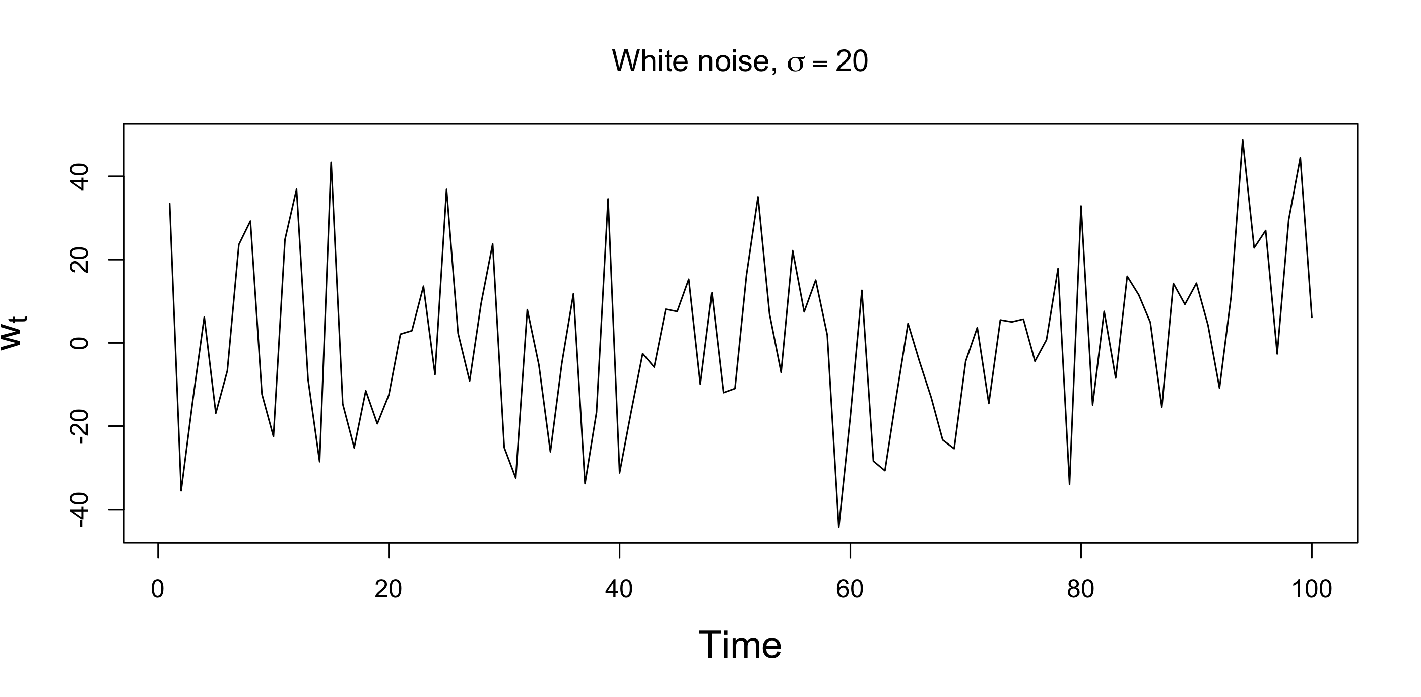
The first-order autoregressive process, denoted AR(1), is \[ \varepsilon_t = \rho \varepsilon_{t-1} + w_t \] where \(w_t\) is a strictly stationary and ergodic white noise process with 0 mean and variance \(\sigma^2_w\).
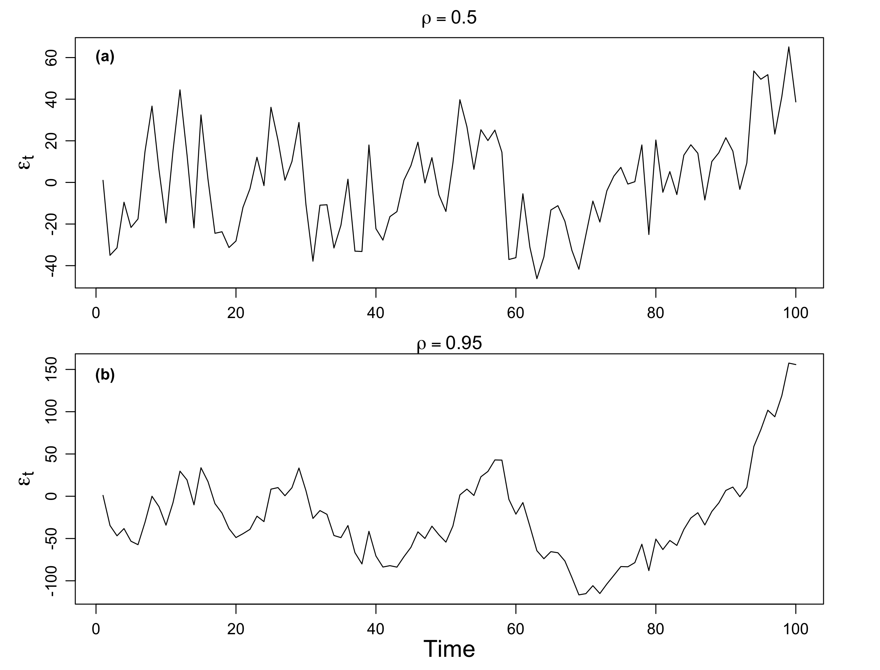
To illustrate the behavior of the AR(1) process, Figure 4.2 plots two simulated AR(1) processes. Each is generated using the white noise process et displayed in Figure 4.1.
The plot in Figure 4.2(a) sets \(\rho=0.5\) and the plot in Figure 4.2(b) sets \(\rho=0.95\).
Remarks
- Figure 4.2(b) is more smooth than Figure 4.2(a).
- The smoothing increases with \(\rho\).
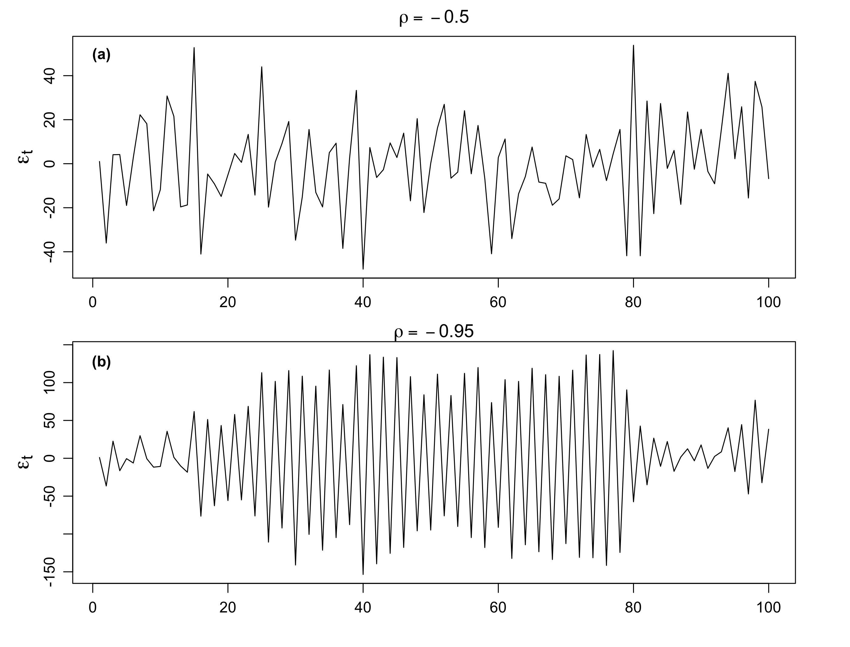
We have seen the cases when \(\rho\) is positive, now let’s consider when \(\rho\) is negative. Figure 4.3(a) shows an AR(1) process with \(\rho=-0.5\), and Figure 4.3(a) shows an AR(1) process with \(\rho=-0.95\,.\)
We see that the sample path is very choppy when \(\rho\) is negative. The different patterns for positive and negative \(\rho\)’s are due to their autocorrelation functions (ACFs).
Possible causes of serial correlation: Incomplete or flawed model specification. Relevant factors omitted from the time series regression are correlated across periods.
4.3 Mathematical Representation
Let’s formulate an AR(1) model as follows:
\[ \begin{align} \varepsilon_t = \rho \varepsilon_{t-1} + w_t \end{align} \tag{4.1}\]
where \(w_t\) is a white noise series with mean zero and variance \(\sigma^2_w\). We also assume \(|\rho|<1\).
We can represent the AR(1) model as a linear combination of the innovations \(w_t\).
By iterating backwards \(k\) times, we get
\[ \begin{aligned} \varepsilon_t &= \rho \,\varepsilon_{t-1} + w_t \\ &= \rho\, (\rho \, \varepsilon_{t-2} + w_{t-1}) + w_t \\ &= \rho^2 \varepsilon_{t-2} + \rho w_{t-1} + w_t \\ &\quad \vdots \\ &= \rho^k \varepsilon_{t-k} + \sum_{j=0}^{k-1} \rho^j \,w_{t-j} \,. \end{aligned} \] This suggests that, by continuing to iterate backward, and provided that \(|\rho|<1\) and \(\sup_t \text{Var}(\varepsilon_t)<\infty\), we can represent \(\varepsilon_t\) as a linear process given by
\[ \color{#EE0000FF}{\varepsilon_t = \sum_{j=0}^\infty \rho^j \,w_{t-j}} \,. \]
4.3.1 Expectation
\(\varepsilon_t\) is stationary with mean zero.
\[ E(\varepsilon_t) = \sum_{j=0}^\infty \rho^j \, E(w_{t-j}) \]
4.3.2 Autocovariance
The autocovariance function of the AR(1) process is \[ \begin{aligned} \gamma (h) &= \text{Cov}(\varepsilon_{t+h}, \varepsilon_t) \\ &= E(\varepsilon_{t+h}, \varepsilon_t) \\ &= E\left[\left(\sum_{j=0}^\infty \rho^j \,w_{t+h-j}\right) \left(\sum_{k=0}^\infty \rho^k \,w_{t-k}\right) \right] \\ &= \sum_{l=0}^{\infty} \rho^{h+l} \rho^l \sigma_w^2 \\ &= \sigma_w^2 \cdot \rho^{h} \cdot \sum_{l=0}^{\infty} \rho^{2l} \\ &= {\color{red} \frac{\sigma_w^2 \cdot \rho^{h} }{1-\rho^2} }, \quad h>0 \,. \end{aligned} \] When \(h=0\), \[ {\color{red} \gamma(0) = \var(\varepsilon_t) = \frac{\sigma_w^2}{1-\rho^2}} \] is the variance of the process \(\text{Var}(\varepsilon_t)\).
Note that
- \(\gamma(0) \ge |\gamma (h)|\) for all \(h\). Maximum value at 0 lag.
- \(\gamma (h)\) is symmetric, i.e., \(\gamma (-h) = \gamma (h)\)
The autocovariance matrix is
\[ \begin{aligned} \bOmega &= \frac{\sigma_w^2}{1-\rho^2} \begin{bmatrix} 1 & \rho & \cdots & \rho^{n-1} \\ \rho & 1 & \cdots & \rho^{n-2} \\ \vdots & \vdots & \ddots & \vdots \\ \rho^{n-1} & \rho^{n-2} & \cdots & 1 \\ \end{bmatrix} \\ &= \gamma(0)\mathbf{R} \\ &= \bOmega (\rho) \end{aligned} \]
The covariance matrix (\(\bOmega\)) equals the variance (\(\gamma(0)\)) times the autocorrelation matrix (\(\mathbf{R}\)).
Note that \(\gamma(h)\) is never zero, but it does become negligible if \(\abs{\rho}<1.\) That is, the influence of a given disturbance fades as it recedes into the more distant past but vanishes only asymptotically.
4.3.3 Autocorrelation
The autocorrelation function (ACF) is given by
\[ {\color{#337ab7} \rho(h) = \frac{\gamma (h)}{\gamma (0)} = \rho^h }, \] which is simply the correlation between \(\varepsilon_{t+h}\) and \(\varepsilon_{t}\,.\)
The autocorrelation of the stationary AR(1) 24.3 is a simple geometric decay (\(\abs{\rho}<1\)):
- If \(\abs{\rho}\) is small, the autocorrelations decay rapidly to zero with \(h\)
- If \(\abs{\rho}\) is large (close to unity), then the autocorrelations decay moderately
- The AR(1) parameter \(\abs{\rho}\) describes the persistence in the time series
Note that \(\rho(h)\) satisfies the recursion \[ \rho(h) = \rho\cdot \rho(h-1) \,. \]
- For \(\rho >0\), \(\rho(h)=\rho^h>0\) observations close together are positively correlated with each other. The larger the \(\rho\), the larger the correlation.
- For \(\rho <0\), the sign of the ACF \(\rho(h)=\rho^h\) depends on the time interval.
- When \(h\) is even, \(\rho(h)\) is positive;
- when \(h\) is odd, \(\rho(h)\) is negative.
- For example, if an observation, \(\varepsilon_t\), is positive, the next observation, \(\varepsilon_{t+1}\), is typically negative, and the next observation, \(\varepsilon_{t+2}\), is typically positive. Thus, in this case, the sample path is very choppy.
Another interpretation of \(\rho(h)\) is the optimal weight for scaling \(\varepsilon_t\) into \(\varepsilon_{t+h}\), i.e., the weight, \(a\), that minimizes \(E[(\varepsilon_{t+h} - a\,\varepsilon_{t})^2]\,.\)
References
- Chap 19 Models with Lagged Variables, Econometric Analysis, Greene 5th Edition, pp 558.