3.11 Tables

Cross reference tables

Using bookdown cmd: \@ref(tab:chunk-label).

Note that you must provide caption option in knitr::kable(). Otherwise the table won’t be numbered.

And see Table \@ref(tab:mtcars).

```{r mtcars, echo=FALSE}
knitr::kable(mtcars[1:5, 1:5], caption = "The mtcars data.")
```

Refer to the Table 3.1.

Table 3.1: The mtcars data.
	mpg	cyl	disp	hp	drat
Mazda RX4	21.0	6	160	110	3.90
Mazda RX4 Wag	21.0	6	160	110	3.90
Datsun 710	22.8	4	108	93	3.85
Hornet 4 Drive	21.4	6	258	110	3.08
Hornet Sportabout	18.7	8	360	175	3.15

knitr::kable(x, format="pipe") is useful when you want to copy-and-paste R output from console to other document, e.g., markdown.

knitr::kable(mtcars[1:5, 1:5], format = "pipe")
|                  |  mpg| cyl| disp|  hp| drat|
|:-----------------|----:|---:|----:|---:|----:|
|Mazda RX4         | 21.0|   6|  160| 110| 3.90|
|Mazda RX4 Wag     | 21.0|   6|  160| 110| 3.90|
|Datsun 710        | 22.8|   4|  108|  93| 3.85|
|Hornet 4 Drive    | 21.4|   6|  258| 110| 3.08|
|Hornet Sportabout | 18.7|   8|  360| 175| 3.15|

3.11.1 `knitr::kable`

knitr::kable(x, digits, caption=NULL, escape=TRUE) Create tables in LaTeX, HTML, Markdown and reStructuredText.

It adjusts column widths automatically based on content.

caption The table caption. In order to number the table, mut specify the caption argument.
format Possible values are latex, html, pipe (Pandoc’s pipe tables), simple (Pandoc’s simple tables), rst, and jira.

The value of this argument will be automatically determined if the function is called within a knitr document.
digits Maximum number of digits for numeric columns, passed to round().
col.names Rename columns.
escape = TRUE Whether to escape special characters when producing HTML or LaTeX tables.

Default is TRUE, will treat characters literally; special characters will either be escaped or substituted; no special characters will be interpreted.

For example, $ is escaped as \$, _ is escaped as \_, and \ is substituted with \textbackslash{}

See Math in rmd tables for examples of using math symbols in rmd tables.
- Set escape = FALSE when you have math symbols in the table.
  
  It makes sure that the math symbols will be rendered.
  
  Note that you need to escape certain special characters in LaTeX math mode though, e.g., use \\sigma for printing $\sigma$ in kable.
  - Don’t need to escape $, ^ and _ in math mode.
- When set to FALSE, you have to make sure yourself that special characters will not trigger syntax errors in LaTeX or HTML.
- Common special LaTeX characters include #, %, &, {, and }. Common special HTML characters include &, <, >, and ". These can easily lead to errors or unexpected effects when you render your file.
align Column alignment: a character vector consisting of 'l' (left), 'c' (center) and/or 'r' (right).
- By default or if align = NULL, numeric columns are right-aligned, and other columns are left-aligned.
  
  文字列左对齐，数字列右对齐。
- If only one character is provided, that will apply to all columns.
- If a vector is provided, will map to each individual column specifically.
Missing values (NA) in the table are displayed as NA by default.

If you want to display them with other characters, you can set the option knitr.kable.NA, e.g. options(knitr.kable.NA = '') in the YAML to hide NA values.

booktabs = TRUE use the booktabs package. Default to FALSE.

`booktabs`	`True`	`FALSE`
Column separator	No vertical lines in the table, you can add via `vline` option	Table columns are separated by vertical lines.
Horizontal lines	Only has horizontal lines for the table header and the bottom row. - Use `\toprule`, `\midrule`, and `\bottomrule`	Use `\hline`
Row behavior	A line space is added to every five rows by default. Disable it with `linesep = ""`.

linesep = "" remove the extra space after every five rows in kable output (with booktabs option)

linesep = c("", "", "", "", "\\addlinespace") default value; empty line space every 5 rows.

# For Markdown tables, use `pipe` format
> knitr::kable(head(mtcars[, 1:4]), format = "pipe")
|                  |  mpg| cyl| disp|  hp|
|:-----------------|----:|---:|----:|---:|
|Mazda RX4         | 21.0|   6|  160| 110|
|Mazda RX4 Wag     | 21.0|   6|  160| 110|
|Datsun 710        | 22.8|   4|  108|  93|
|Hornet 4 Drive    | 21.4|   6|  258| 110|
|Hornet Sportabout | 18.7|   8|  360| 175|
|Valiant           | 18.1|   6|  225| 105|

# For Plain tables in txt, `simple` is useful
> knitr::kable(head(mtcars[, 1:4]), format = "simple") 
                      mpg   cyl   disp    hp
------------------  -----  ----  -----  ----
Mazda RX4            21.0     6    160   110
Mazda RX4 Wag        21.0     6    160   110
Datsun 710           22.8     4    108    93
Hornet 4 Drive       21.4     6    258   110
Hornet Sportabout    18.7     8    360   175
Valiant              18.1     6    225   105

3.11.1.1 Math in rmd tables

knitr::kable(x, escape=TRUE)

escape=TRUE whether to escape special characters when producing HTML or LaTeX tables. Refer to kable arguments for more details.
- Defaults to TRUE.
- When escape = FALSE, you have to make sure that special characters will not trigger syntax errors in LaTeX or HTML. E.g., if you don’t escape \, it will cause an error.

You need to escape backslashes (\) passed into the table data.

Example 1 of escaping special characters:

```{r, echo=FALSE}
library(knitr)

mathy.df <- data.frame(site = c("A", "B"), 
                       b0 = c(3, 4), 
                       BA = c(1, 2))

colnames(mathy.df) <- c("Site", "$\\beta_0$", "$\\beta_A$")

kable(mathy.df, escape=FALSE)
```

If your target output is pdf, it is possible to edit Latex table directly in Rmd.

Don’t enclose in $$.
Use \begin{table} and start your table data.

Example 2 of escaping special characters:

library(knitr)

df <- data.frame(
  Variable = c("Return", "Variance", "Literal symbols"),
  Formula = c("$r_t = \\frac{P_t}{P_{t-1}} - 1$", 
              "$\\sigma^2 = Var(r_t)$",
              "\\$, \\%, \\_, \\#")
)

kable(df, escape = FALSE, booktabs = TRUE)

Variable	Formula
Return	$r_t = \frac{P_t}{P_{t-1}} - 1$
Variance	$\sigma^2 = Var(r_t)$
Literal symbols	$, %, _, #

Expected behaviors:

Return row → LaTeX math $r_t ...$ renders properly.
Variance row → works with superscripts and variance notation.
Literal symbols row → shows $ % _ # as text in the PDF.

3.11.2 Data frame printing

To show the tibble information (number of row/columns, and group information) along with paged output, we can write a custom function by modifying the print.paged_df function (which is used internally by rmarkdown for the df_print feature) and use CSS to nicely format the output.

https://stackoverflow.com/a/76014674/10108921

Paged df

---
title: "Use caption with df_print set to page"
date: "2025-09-29"
output:
  bookdown::html_document2:
    df_print: paged
---

When the df_print option is set to paged, tables are printed as HTML tables with support for pagination over rows and columns.

The possible values of the df_print option for the html_document format.

Option	Description
`default`	Call the `print.data.frame` generic method; console output prefixed by `##`;
`kable`	Use the `knitr::kable` function; looks nice but with no navigation for rows and columns, neither column types. Suggested for pdf output.
`tibble`	Use the `tibble::print.tbl_df` function, this provides groups and counts of rows and columns info as if printing a `tibble`.
`paged`	Use `rmarkdown::paged_table` to create a pageable table; `paged` looks best but slows down compilation significantly;
A custom function	Use the function to create the table

The possible values of the df_print option for the pdf_document format: default, kable, tibble, paged, or a custom function.

paged print

```{r echo=TRUE, paged.print=TRUE}
ggplot2::diamonds
```

default output

```{r echo=TRUE, paged.print=FALSE}
ggplot2::diamonds
```

kable output

```{r echo=TRUE}
knitr::kable(ggplot2::diamonds[1:10, ])
```

Note that kable output doesn’t provide tibble information.

Available options for paged tables:

Option	Description
max.print	The number of rows to print.
rows.print	The number of rows to display.
cols.print	The number of columns to display.
cols.min.print	The minimum number of columns to display.
pages.print	The number of pages to display under page navigation.
paged.print	When set to `FALSE` turns off paged tables.
rownames.print	When set to `FALSE` turns off row names.

These options are specified in each chunk like below:

```{r cols.print=3, rows.print=3}
mtcars
```

For pdf_document, it is possible to write LaTex code directly.

```{=latex}
\begin{tabular}{ll}
A & B \\
A & B \\
\end{tabular}
```

Do not forget the equal sign before latex, i.e., it is =latex instead of latex.

3.11.3 Stargazer

stargazer print nice tables in Rmd documents and R scripts:

Passing a data frame to stargazer package creates a summary statistic table.
Passing a regression object creates a nice regression table.
Support tables output in multiple formats: text, latex, and html.
- In R scripts, use type = "text" for a quick view of results.
stargaer does NOT work with anova table, use pander::pander instead.

3.11.3.1 Text table

Specify stargazer(model, type = "text")

```{r descrptive-analysis-text, comment = ''}
apply(data[,-1], 2, get_stat) %>% 
    stargazer(type = "text", digits = 2)
```

The text output looks like the following.

===============================================
                        Dependent variable:    
                    ---------------------------
                            delta_infl         
-----------------------------------------------
unemp                         -0.091           
                              (0.126)          
                                               
Constant                       0.518           
                              (0.743)          
                                               
-----------------------------------------------
Observations                    203            
R2                             0.003           
Adjusted R2                   -0.002           
Residual Std. Error      2.833 (df = 201)      
F Statistic             0.517 (df = 1; 201)    
===============================================
Note:               *p<0.1; **p<0.05; ***p<0.01

Significance codes are shown in the footnote.

By default, stargazer uses ***, **, and * to denote statistical significance at the one, five, and ten percent levels (* p<0.1; ** p<0.05; *** p<0.01).
In contrast, summary.lm uses * p<0.05, ** p<0.01, *** p< 0.001.
You can change the cutoffs for significance using star.cutoffs = c(0.05, 0.01, 0.001).

There is one empty line after each coefficient, to remove the empty lines, specify no.space = TRUE.

The regression table with all empty lines removed:

===============================================
                        Dependent variable:    
                    ---------------------------
                            delta_infl         
-----------------------------------------------
unemp                         -0.091           
                              (0.126)          
Constant                       0.518           
                              (0.743)          
-----------------------------------------------
Observations                    203            
R2                             0.003           
Adjusted R2                   -0.002           
Residual Std. Error      2.833 (df = 201)      
F Statistic             0.517 (df = 1; 201)    
===============================================
Note:               *p<0.1; **p<0.05; ***p<0.01

3.11.3.2 HTML table

HTML table can be obtained by specifying stargazer(model, type = "html").

Note that you need to specify results="asis" in the code chunk options. This option tells knitr to treat verbatim code blocks “as is.” Otherwise, instead of your table, you will see the raw html or latex code.

Note that *’s do NOT show properly in html output, see Fig. 3.10, need to specify in the footnote (notes) manually.

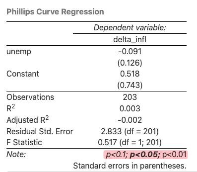
Figure 3.10: Failed to show significance codes in HTML output.

Use the following code to display the correct significance symbols.

```{r descrptive-analysis-html, results="asis"}
# the following code fixes the significance codes in html output
apply(data[,-1], 2, get_stat) %>% 
    stargazer(
      type = "html", digits = 2, 
      notes = "<span>&#42;</span>: p<0.1; <span>&#42;&#42;</span>: <strong>p<0.05</strong>; <span>&#42;&#42;&#42;</span>: p<0.01 <br> Standard errors in parentheses.",
      notes.append = F
      )
```

* is the HTML entity code for *.
Stargazer by default using * for 10% significance, ** for 5% significance, and *** for 1% significance.

After correcting the significance codes, the output looks like Fig. 3.11.

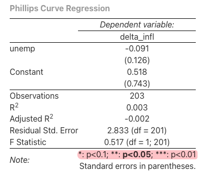
Figure 3.11: Correct significance codes.

3.11.3.3 Common arguments

Table general formatting options:

type = "latex" | "html" | "text" specify output table format.
digits = 3 an integer that indicates how many decimal places should be used. Defaults to 3 digits.

A value of NULL indicates that no rounding should be done at all, and that all available decimal places should be reported.
notes a character vector containing notes to be included below the table.
notes.append = FALSE a logical value that indicates whether notes should be appended to the existing standard note(s) associated with the table’s style (typically an explanation of significance cutoffs).
- Defaults to TRUE.
- If the argument’s value is set to FALSE, the character strings provided in notes will replace any existing/default notes.
notes.align: "l" for left alignment, "r" for right alignment, and "c" for centering. This argument is not case-sensitive.

Control structure of regression tables

intercept.bottom = TRUE place the intercept at the bottom of the table.
keep.stat = NULL: control which model statistics should be kept in the table. Possible values include "n", "rsq", "adj.rsq", "f", "ser", "ll", "aic", "bic", and "logLik".
- The default is NULL, which means that all available statistics will be included in the table.
- To exclude all statistics, set keep.stat = c().
- To include only the number of observations and the adjusted R-squared, set keep.stat = c("n", "adj.rsq").

Make your model names more informative:

column.separate a numeric vector that specifies how column.labels should be laid out (grouped) across regression table columns.

A value of c(2, 1, 3), for instance, will apply the first label to the two first columns, the second label to the third column, and the third label will apply to the following three columns (i.e., columns number four, five and six).
dep.var.labels labels for dependent variables.
column.labels a character vector of labels for columns in regression tables.

This is useful to denote different regressions, informing the name/nature of the model, instead of using numbers to identify them.

When you add custom column labels, you may want to use: model.numbers = FALSE to suppress the default model numbers (1) (2)…

covariate.labels labels for covariates in the regression tables.

Can provide latex symbols in the labels, need to escape special symbols though.

stargazer(mod_sel_lm_mtcars, 
          covariate.labels = 
            c("(Intercept)", "drat", "hp", "$w_{i}$",
              "\\textit{k}", "logLik", "AICc", "\\Delta AICc"))

add.lines add a row(s) for additional info, such as reporting fixed effects.

stargazer(output, output2, type = "html",
          add.lines = list(
            c("Fixed effects?", "No", "No"),
            c("Results believable?", "Maybe", "Try again later")
            )
          )

Make your table more compact:

single.row = TRUE to put coefficients and standard errors on same line
no.space = TRUE to remove the spaces after each line of coefficients
font.size = "small" to make font size smaller

Tip: Add a blank line under the stargazer table:   with a blank line above and below.

3.11.3.4 Cross reference `stargazer` tables

In pdf output, use Table \@ref(tab:reg-table) or Table \ref{tab:reg-table}.
```
Table \@ref(tab:reg-table) summarize the regression results in a table.

```{r, include=TRUE, results='asis'}
stargazer(capm_ml, FF_ml, type='latex', header=FALSE,
          digits=4, no.space = TRUE,
          title="Regression Results for META",
          label = "tab:reg-table")
```
```
❗️ Note that you need to specify results="asis" in the code chunk options. Omitting this options will result in failing to compile tex.
- header=FALSE is to suppress the % Table created by stargazer header. This applies to only latex tables.
```
% Table created by stargazer v.5.2.3 by Marek Hlavac, Social Policy Institute. E-mail: marek.hlavac at gmail.com
% Date and time: Fri, Sep 19, 2025 - 15:16:36
```
- label="tab:reg-table" is to specify the cross reference label for the table.
- table.placement = "H" set float to H to fix positions. Places the float at precisely the location in the code. This requires the float LaTeX package. Remember to load it in the YAML.
  - Defaults to "!htbp".
    
    The htbp controls where the table or figure is placed. Tables and figures do not need to go where you put them in the text. LATEX moves them around to prevent large areas of white space from appearing in your paper. h (Here): Place the float here, i.e., approximately at the same point it occurs in the source text (however, not exactly at the spot) t (Top): Place the table at the top of the current page b (Bottom): Place the table at the bottom of the current page. p (Page): Place the table at the top of the next page. !: Override internal parameters LaTeX uses for determining “good” float positions.
- align = FALSE a logical value indicating whether numeric values in the same column should be aligned at the decimal mark in LaTeX output.

In html output, cross references to stargazer tables are NOT so straightforward.

label option in stargazer does not work. Cannot use chunk labels either.

```{r fit-age, echo=FALSE, results='asis', fig.cap="Logistic regression of CHD on age."}
# Use title caption from fig.cap
tit <- knitr::opts_current$get("fig.cap")
# Adding caption for html output
tit_html <- paste0(
  '<span id="tab:', knitr::opts_current$get("label"),'">(#tab:',
        knitr::opts_current$get("label"), ')</span>', tit)
stargazer::stargazer(fit.age,
          label = paste0("tab:", knitr::opts_current$get("label")),
          title = ifelse(knitr::is_latex_output(), tit, tit_html),
          type = ifelse(knitr::is_latex_output(),"latex","html"),
          notes = "<span>&#42;</span>: p<0.1; <span>&#42;&#42;</span>: <strong>p<0.05</strong>; <span>&#42;&#42;&#42;</span>: p<0.01 <br> Standard errors in parentheses.",
          notes.append = F,
          header = F
          )
```

Here is another reference to stargazer Table \@ref(tab:fit-age).

Don’t change things unless it is absolutely necessary. Run the code chunk before compiling the whole website. It gets slowly as the website gets larger.

stargazer::stargazer() the :: is necessary, and header=F is necessary and should be place at the end, otherwise will have errors as follows.

Error in `.stargazer.wrap()`:
! argument is missing, with no default
Backtrace:
 1. stargazer::stargazer(...)
 2. stargazer:::.stargazer.wrap(...)
Execution halted

Exited with status 1.

Another example if you don’t need to add footnotes.

```{r mytable, results='asis', fig.cap="This is my table."}

# Use title caption from fig.cap
tit <- knitr::opts_current$get("fig.cap")

# Adding caption for html output
tit_html <- paste0('<span id="tab:',
                   knitr::opts_current$get("label"),
                   '">(#tab:',
                   knitr::opts_current$get("label"),
                   ')</span>',
                   tit)

stargazer::stargazer(
  fit.age,
  label = paste0("tab:", knitr::opts_current$get("label")),
  title = ifelse(knitr::is_latex_output(), tit, tit_html),
  type = ifelse(knitr::is_latex_output(),"latex","html"),
  header = F
  )
```

Here is a reference to stargazer Table \@ref(tab:mytable).

Alignment of Stargazer Tables

In PDF, the tables will be in the center by default.
However, when working with HTML output, you need to add CSS styling to adjust the table.

References:

https://libguides.princeton.edu/c.php?g=1326286&p=9763596#s-lg-box-wrapper-36305037

3.11.4 `xtable`

Two steps:

convert to xtable object
print to LaTeX or html code

xtab <- xtable(tableResults, caption = NULL, digits = NULL)
print(xtab, include.rownames=FALSE)

xtable converts an R object to an xtable object, which can then be printed as a LaTeX or HTML table.

xtable() arguments

align Character vector of length equal to the number of columns of the resulting table, indicating the alignment of the corresponding columns. Also, "|" may be used to produce vertical lines between columns in LaTeX tables, but these are effectively ignored when considering the required length of the supplied vector.
- If a character vector of length one is supplied, it is split as strsplit(align, "")[[1]] before processing. Since the row names are printed in the first column, the length of align is one greater than ncol(x) if x is a data.frame.
- Use "l", "r", and "c" to denote left, right, and center alignment, respectively.
- Use "p{3cm}" etc. for a LaTeX column of the specified width. For HTML output the "p" alignment is interpreted as "l", ignoring the width request. Default depends on the class of x.
caption Character vector of length 1 or 2 containing the table’s caption or title. If length is 2, the second item is the “short caption” used when LaTeX generates a “List of Tables”.
digits Numeric vector of length equal to one (in which case it will be replicated as necessary) or to the number of columns of the resulting table or matrix of the same size as the resulting table, indicating the number of digits to display in the corresponding columns.

print.xtable() arguments

include.rownames A logical value indicating whether the row names of x should be printed. Default is TRUE.
type Possible values are "latex" and "html". Default is "latex".

Print a data frame

library(xtable)

df <- data.frame(
  Asset = c("A", "B"),
  Mu = c(0.175, 0.055),
  Sigma = c(0.258, 0.115)
)

# Convert to xtable
xtab <- xtable(df, caption = "Asset Parameters", digits = 3)

# Print html code
print(xtab, type = "html", include.rownames = TRUE)

Asset Parameters
	Asset	Mu	Sigma
1	A	0.175	0.258
2	B	0.055	0.115

Print a regression table

model <- lm(mpg ~ hp + wt, data = mtcars)
xtab_model <- xtable(model, caption = "Regression of mpg on hp and wt")

# Print as html
print(xtab_model, type = "html", digits = 3)

Regression of mpg on hp and wt
	Estimate	Std. Error	t value	Pr(>\|t\|)
(Intercept)	37.2273	1.5988	23.28	0.0000
hp	-0.0318	0.0090	-3.52	0.0015
wt	-3.8778	0.6327	-6.13	0.0000

3.11.5 `kableExtra`

The kableExtra package is designed to extend the basic functionality of tables produced using knitr::kable().

kableExtra::kbl() extends knitr::kable(), with some additional features.

# pipe kabe output to the styling function of kableExtra
kable(iris) %>%
  kable_styling(latex_options = "striped")

kableExtra::kable_styling(bootstrap_options = c("striped", "hover"), full_width = FALSE)

bootstrap_options A character vector for bootstrap table options. Please see package vignette or visit the w3schools’ Bootstrap Page for more information. Possible options include basic, striped, bordered, hover, condensed, responsive and none.
- striped alternating row colors
- hover Use the :hover selector on tr (table row) to highlight table rows on mouse over.
full_width A TRUE or FALSE variable controlling whether the HTML table should have 100% the preferable format for full_width. If not specified,
- TRUE for a HTML table , will have full width by default but
- this option will be set to FALSE for a LaTeX table.

latex_options A character vector for LaTeX table options, i.e., won’t have effect on html tables.

Possible options:

Arguments	Meanings
`striped`	Add alternative row colors to the table. It will imports `LaTeX` package `xcolor` if enabled.
`scale_down`	useful for super wide table. It will automatically adjust the table to fit the page width.
`repeat_header`	only meaningful in a long table environment. It will let the header row repeat on every page in that long table.
`hold_position`	“hold” the floating table to the exact position. It is useful when the `LaTeX` table is contained in a `table` environment after you specified captions in `kable()`. It will force the table to stay in the position where it was created in the document.
`HOLD_position`	A stronger version of `hold_position`. Requires the float package and specifies ⁠[H]⁠.

Rows and columns can be grouped via the functions pack_rows() and add_header_above(), respectively.

scroll_box(width = "100%", height = "500px") let you create a fixed height table while making it scrollable. This function only works for html long tables.

# commonly used settings 
table %>% 
    knitr::kable(digits = 5) %>%
    kable_styling(bootstrap_options = c("striped", "hover"), full_width = FALSE, latex_options="scale_down") %>% 
    scroll_box(width = "100%", height = "500px")

# escape=TRUE, this makes your life easier, will output the table exactly as it is
result <- read_csv("~/Documents/GDP/data/reg_result/IFE_result.csv")
result %>%
  knitr::kable(digits = 5, escape=T) %>%
  kable_styling(bootstrap_options = c("striped", "hover"), full_width = FALSE, latex_options="scale_down")

# escape=FALSE, have to specify escape by replace `*` to `\\\\*`
result <- read_csv("~/Documents/GDP/data/reg_result/IFE_result.csv")
result <- result %>% 
  mutate(pval.symbol = gsub("[*]", "\\\\*", pval.symbol) )
result %>%
  knitr::kable(digits = 5, escape=FALSE) %>%
  kable_styling(bootstrap_options = c("striped", "hover"), full_width = FALSE, latex_options="scale_down")

3.11.5.1 tables in pdf output

reg_data %>% 
    select(Date, adjusted, eRi, rmrf) %>%
    head(10) %>% 
    knitr::kable(digits = c(0,2,4,4), escape=T, format = "latex", booktabs = TRUE, linesep = "" ) %>%
    kable_styling(latex_options = c("striped"), full_width = FALSE, stripe_color = "gray!15")

knitr::kable() arguments

format = "latex" specifies the output format.
align = "l" specifies column alignment.
booktabs = TRUE is generally recommended for formatting LaTeX tables.
linesep = "" prevents default behavior of extra space every five rows.

kableExtra::kable_styling() arguments

position = "left" places table on left hand side of page.
latex_options = c("striped", "repeat_header") implements table striping with repeated headers for tables that span multiple pages.
stripe_color = "gray!15" species the stripe color using LaTeX color specification from the xcolor package - this specifies a mix of 15% gray and 85% white.

linebreak(x, align = "l", double_escape = F, linebreaker = "\n") Make linebreak in LaTeX Table cells.

align="l" Choose from “l”, “c” or “r”. Defaults to “l”.

3.11.5.2 Customize the looks for columns/rows

kableExtra::column_spec(kable_input, column) this function allows users to select a column and then specify its look.

# specify the width of the first two columns to be 5cm
table %>%
  knitr::kable() %>%
  column_spec(1:2, width = "5cm")

kable_input: Output of knitr::kable()
column: A numeric value or vector indicating which column(s) to be selected.

E.g., to format the 1st and 3rd columns: column_spec(c(1, 3), width = "5cm").

row_spec() works similar with column_spec() but defines specifications for rows.

For the position of the target row, you don’t need to count in header rows or the group labeling rows.
row_spec(row = 0, align='c') specify format of the header row. Here I want to center align headers.

3.11.5.3 Add header rows to group columns

add_header_above(): The header variable is supposed to be a named character with the names as new column names and values as column span.

For your convenience, if column span equals to 1, you can ignore the =1 part so the function below can be written as add_header_above(c("", "Group 1" = 2, "Group 2" = 2, "Group 3" = 2)).

kbl(dt) %>%
  kable_classic() %>%
  add_header_above(c(" " = 1, "Group 1" = 2, "Group 2" = 2, "Group 3" = 2))

You can add another row of header on top.

3.11.5.4 Group rows

collapse_rows will put repeating cells in columns into multi-row cells. The vertical alignment of the cell is controlled by valign with default as “top”.

Not working for html output.

collapse_rows_dt <- data.frame(C1 = c(rep("a", 10), rep("b", 5)),
                 C2 = c(rep("c", 7), rep("d", 3), rep("c", 2), rep("d", 3)),
                 C3 = 1:15,
                 C4 = sample(c(0,1), 15, replace = TRUE))

kableExtra::kbl(collapse_rows_dt, align = "c") %>%
  kable_paper(full_width = F) %>%
  column_spec(1, bold = T) %>%
  collapse_rows(columns = 1:2, valign = "top")

Empty string as column name in tibble: use setNames or attr

df <- tibble(" "=1)
setNames(df, "")
# # A tibble: 1 x 1
#      ``
#   <dbl>
# 1     1

attr(df, "names") <- c("")

footnote() add footnotes to tables.

There are four notation systems in footnote, namely general (no prefix for footnotes), number, alphabet and symbol.

3.11.6 huxtable

huxtable supports export to LaTeX, HTML, Microsoft Word, Microsoft Excel, Microsoft Powerpoint, RTF and Markdown.

Changing layout

library(tidyverse)
library(huxtable)
df <- data.frame(
  Parameter = c("\\( \\mu \\)", "\\( \\sigma^2 \\)"),
  Boeing = c(0.149, 0.069),
  Microsoft = c(0.331, 0.136)
)
ht <- as_hux(df)
ht <- ht %>% 
  insert_row("\\( \\rho \\)(Boeing, Microsoft)", -0.008, "", after=3) %>% 
  merge_cells(4, 2:3) %>% 
  set_align(4, 2:3, "center") %>%
  set_bold(1, everywhere, TRUE) %>%
  set_width(0.6)

# print_latex(ht) # uncomment this line if printing as LaTeX table
print_html(ht) # print as HTML table

Parameter	Boeing	Microsoft
$\mu$	0.149	0.331
$\sigma^2$	0.069	0.136
$\rho$(Boeing, Microsoft)	-0.008

as_hux() convert a data frame to a huxtable object.
insert_row(..., after) insert a new row after the specified row number.

Need to provide values for all columns. Empty values can be filled with "".
Table header as row 1
- insert a new row 3 would be after = 3.
- insert as the first row would be after = 0.
merge_cells(row, col) merge cells in the specified rows and columns.
set_align(row, col, value) set alignment for the specified rows and columns.
- set_align("center") set all cells to be center aligned.
set_width(value) set the width of the table. Default html tables are 100% width.

A numeric width is treated as a proportion of f the surrounding block width (HTML) or text width (LaTeX).
col_width(ht, value) set relative widths for each column.
```
col_width(jams) <- c(.2, .8)
```
Math symbols works fine for bookdown, but not for xaringan presentations.
- By default, huxtable will escape special characters in your cells.
  - To display special characters such as LaTeX maths, set the escape_contents property to FALSE.
  - Alternatively, manually escape special characters.
    
    Use \$ \\mu \$, \\$ does not work.
- For xaringan, use unicode symbols instead, e.g., μ for \mu, σ for \sigma, and ρ for \rho.

Example with math symbols in huxtable:

set_escape_contents(FALSE) to turn off escaping special characters.
Set code chunk option results='asis' to print the table as is.
Escape backslash \ with another backslash \\.

# set escape_contents to FALSE
df <- data.frame(
  Parameter = c("$\\mu$", "$\\sigma^2$"),
  Boeing = c(0.149, 0.069),
  Microsoft = c(0.331, 0.136)
)
ht <- as_hux(df) %>% 
  set_escape_contents(FALSE) %>%    # turn off escaping special characters
  set_align("center") %>%           # center align all cells
  set_bold(1, everywhere, TRUE) %>% # bold header row
  set_width(0.6)                    # set table width
print_html(ht)

Parameter	Boeing	Microsoft
$\mu$	0.149	0.331
$\sigma^2$	0.069	0.136

In xaringan presentations, use unicode symbols instead of LaTeX math symbols.

In xaringan presentations, table width is automatically adjusted to fit contents.
In html output, table width is 100% by default.

```{r results='asis'} 
# Create huxtable and use special characters that will be converted to math
df <- data.frame(
  Parameter = c("μ", "σ²"),
  Boeing = c(0.149, 0.069),
  Microsoft = c(0.331, 0.136)
)
ht <- as_hux(df)
ht <- ht %>% 
  insert_row("ρ(Boeing, Microsoft)", -0.008, "", after=3) %>% 
  merge_cells(4, 2:3) %>% 
  set_width(0.6) %>%
  set_bold(1, everywhere, TRUE) %>%
  set_align(everywhere, everywhere, "center")

print_html(ht)
```

will be render as:

Parameter	Boeing	Microsoft
μ	0.149	0.331
σ²	0.069	0.136
ρ(Boeing, Microsoft)	-0.008

Variable	Formula
Return	\(r_t = \frac{P_t}{P_{t-1}} - 1\)
Variance	\(\sigma^2 = Var(r_t)\)
Literal symbols	$, %, _, #

Parameter	Boeing	Microsoft
\(\mu\)	0.149	0.331
\(\sigma^2\)	0.069	0.136
\(\rho\)(Boeing, Microsoft)	-0.008