8.5 Time Series Regression
Distributed Lag model using dynlm package, which is useful for dynamic linear models and time series regressions. Lags or differences can directly be specified in the model formula.
The main function used to estimate our model is the dynlm(formula, data) function. Within this function, d() can be used to specify the difference in a variable and L() can be used to compute the desired lag of the variable.
d(u, 1) means to calculate the first difference in u; L(g, 0:2) denotes g of the current period and the past two periods, \(g\), \(g_{-1}\), and \(g_{-2}\).
Note that data must be either a data frame or zoo object. xts returns an error.
> library(dynlm)
# Finite Distributed Lag Models
> okun.lag2 <- dynlm(d(unemp, 1) ~ L(gGDP, 0:2), data = okun2.zoo)  # lag 2
> okun.lag3 <- dynlm(d(unemp, 1) ~ L(gGDP, 0:3), data = okun2.zoo)  # lag 3
# ARDL(1, 1)
> okun.ardl <- dynlm(d(unemp, 1) ~ L(d(unemp, 1), 1) + L(gGDP, 0:1), data = okun2.zoo)
> summary(okun.ardl)

Time series regression with "zoo" data:
Start = 1948 Q3, End = 2025 Q1

Call:
dynlm(formula = d(unemp, 1) ~ L(d(unemp, 1), 1) + L(gGDP, 0:1),
    data = okun2.zoo)

Residuals:
    Min      1Q  Median      3Q     Max
-1.4662 -0.2198 -0.0218  0.1686  4.9875

Coefficients:
                  Estimate Std. Error t value Pr(>|t|)
(Intercept)        0.42871    0.03769  11.374  < 2e-16 ***
L(d(unemp, 1), 1) -0.05640    0.05874  -0.960 0.337736
L(gGDP, 0:1)1     -0.43423    0.02390 -18.165  < 2e-16 ***
L(gGDP, 0:1)2     -0.11951    0.03575  -3.343 0.000932 ***
---
Signif. codes:  0 ‘***’ 0.001 ‘**’ 0.01 ‘*’ 0.05 ‘.’ 0.1 ‘ ’ 1

Residual standard error: 0.4416 on 303 degrees of freedom
  (0 observations deleted due to missingness)
Multiple R-squared:  0.5825,    Adjusted R-squared:  0.5784
F-statistic: 140.9 on 3 and 303 DF,  p-value: < 2.2e-16
8.5.1 Lag Polynomial
Let \(\rho(L)=1-\rho_1L\) and \(\beta(L)=\beta_0+\beta_1L.\) Now we have \(\psi(L)\) such at
\[ \rho(L)\psi(L)=\beta(L) . \]
We want to find \(\psi(L)=\rho(L)^{-1}\beta(L).\)
# Compute psi(L) = rho(L)^(-1) * beta(L)
lag_poly_solution <- function(rho1, beta0, beta1, n_terms = 5) {
  # Expand (1 - rho1*L)^(-1) as a power series up to n_terms
  # (1 - rho1*L)^(-1) = 1 + rho1*L + rho1^2*L^2 + ... + rho1^n*L^n
  rho_inv <- sapply(0:n_terms, function(k) rho1^k)

  # beta(L) = beta0 + beta1*L
  # psi(L) = (1 + rho1*L + rho1^2*L^2 + ...)*(beta0 + beta1*L)
  #         = beta0*(1 + rho1*L + ...) + beta1*L*(1 + rho1*L + ...)
  #         = beta0*rho_inv + beta1*c(0, rho_inv[1:n_terms])
  psi <- beta0 * rho_inv
  psi <- psi + beta1 * c(0, rho_inv[1:n_terms])

  # Return coefficients: psi0 + psi1*L + psi2*L^2 + ...
  names(psi) <- paste0("L^", 0:n_terms)
  return(psi)
}
# Example usage:
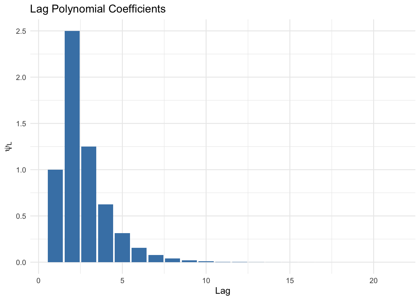
psi_coef <- lag_poly_solution(rho1 = 0.5, beta0 = 1, beta1 = 2, n_terms = 20)
psi_coef## L^0 L^1 L^2 L^3 L^4 L^5
## 1.000000e+00 2.500000e+00 1.250000e+00 6.250000e-01 3.125000e-01 1.562500e-01
## L^6 L^7 L^8 L^9 L^10 L^11
## 7.812500e-02 3.906250e-02 1.953125e-02 9.765625e-03 4.882812e-03 2.441406e-03
## L^12 L^13 L^14 L^15 L^16 L^17
## 1.220703e-03 6.103516e-04 3.051758e-04 1.525879e-04 7.629395e-05 3.814697e-05
## L^18 L^19 L^20
## 1.907349e-05 9.536743e-06 4.768372e-06Plot the lag polynomial coefficients:
library(tidyverse)
psi_df <- tibble(
  lag = 1:21,
  coef = psi_coef
)

# Bar plot
ggplot(psi_df, aes(x = lag, y = coef)) +
  geom_bar(stat = "identity", fill = "steelblue") +
  labs(x = "Lag", y = expression(psi[L]), title = "Lag Polynomial Coefficients") +
  theme_minimal()