5.7 Contingency Table
Confusion tables / contingency tables / crosstabs for analyzing categorical data relationships.
5.7.1 Basic Frequency Counting
The dplyr::count() Function
dplyr::count(x, vars=NULL, wt_var=NULL) lets you quickly count the freqency of unique values of one or more variables. Returns a data.frame.
xdata frame to be processedvarsvariable(s) to count unique values of.If it is one variable, then it returns a frequency table.
It there are two variables, then it returns the count for each possible combination of categories of the two variables. Return a
data.framewith 3 columns. First 2 columns (named after the 2 variables) specify combinations, the third column (Freq) shows the frequency.wt_varoptional variable to weight by - if this is non-NULL, count will sum up the value of this variable for each combination of id variables.
df %>% count(a, b) is roughly equivalent to df %>% group_by(a, b) %>% summarise(n = n()). For each combination of (a,b), count the frequency.
# Count of each value of "id" in the first 100 cases
count(baseball[1:100,], vars = "id")

# Count of ids, weighted by their "g" loading
count(baseball[1:100,], vars = "id", wt_var = "g")

# exercises is a dummay variable in `her.no`
count(hers.no, exercise)
#      exercise     n
# 1        0     1191
# 2        1      841
dplyr::tally() works similarly to count, but you need to do group_by first manually. One step more than count.
df %>% group_by(a,b) %>% tally() is equivalent to df %>% group_by(a,b) %>% summarise(n = n()).
5.7.2 Creating Contingency Tables
The table() Function
- Frequency table if providing one variable
- Cross tabulation table with proportion if providing multiple variables
A relative frequency table can be produced using the function prop.table(x, margin=NULL), which takes a table object as argument:
margin: 1 indicates rows, 2 indicates columns.
Table tutorial: https://cran.r-project.org/web/packages/DescTools/vignettes/TablesInR.pdf
table(..., exclude = if (useNA == "no") c(NA, NaN), useNA = c("no", "ifany", "always"), dnn = list.names(...), deparse.level = 1)
table() is more flexible than count(). table() accepts vectors, lists, data.frames, but count() accepts data.frames only.
...one or more objects which can be interpreted as factors (including character strings), or a list (or data frame) whose components can be so interpreted.
E.x codes:
set.seed(1)
tt <- sample(letters, 100, rep=TRUE)

## using table
table(tt)
tt
a b c d e f g h i j k l m n o p q r s t u v w x y z
2 3 3 3 2 4 6 1 6 5 6 4 7 2 2 2 5 4 5 3 8 4 5 4 3 1
## using tapply
tapply(tt, tt, length)
a b c d e f g h i j k l m n o p q r s t u v w x y z
2 3 3 3 2 4 6 1 6 5 6 4 7 2 2 2 5 4 5 3 8 4 5 4 3 1
Another example:
breaks <- seq(1, 3.5, by=0.5)
labels <- seq(1.25, by=0.5, length.out=length(breaks)-1)
cut(x$TCS_reported, breaks=breaks, labels=labels) %>% table()
# .
# 1.25 1.75 2.25 2.75 3.25
# 3   10    4    5    0
apply(x, 2, function(col) cut(col, breaks=breaks, labels=labels) %>% table())
#      TCS_reported TCS_global_cvt
# 1.25            3              2
# 1.75           10              5
# 2.25            4             11
# 2.75            5              2
# 3.25            0              2
The xtabs() Function
xtabs(formula = ~., data) Create a contingency table from cross-classfifying factors.
We now create a cross-tabulated table to see how occurrences break down across age and gender. Notice we use the cut() function to quickly create 4 arbitrary age groups containing equal numbers of people.
5.7.3 Working with Arrays and Multi-dimensional Tables
The returned table works like an array.
Array Creation and Manipulation
# Define an empty array
a <- array(numeric(), c(2,3,0))

> a
<2 x 3 x 0 array of double>
     [,1] [,2] [,3]
[1,]
[2,]
Note that you need to set at least one dimension to zero, otherwise the array will contain something by definition.
dim can be
- an integer (will coerce to a vector), or
- a vector giving the maximal indices in each dimension.
aperm(a, perm) Transpose an array by permuting its dimensions.
permthe subscript permutation vector, usually a permutation of the integers1:n, wherenis the number of dimensions ofa.
# initialize a 3D arry 2x3x2
> x  <- array(1:12, dim = c(2,3,2))
> x
, , 1

     [,1] [,2] [,3]
[1,]    1    3    5
[2,]    2    4    6

, , 2

     [,1] [,2] [,3]
[1,]    7    9   11
[2,]    8   10   12

# array transpose, from 2x3 to 3x2
> aperm(x, c(2,1,3))
, , 1

     [,1] [,2]
[1,]    1    2
[2,]    3    4
[3,]    5    6

, , 2

     [,1] [,2]
[1,]    7    8
[2,]    9   10
[3,]   11   12
Add data to the array using abind. abind works like rbind/cbind but in a generalized way.
So, as rbind/cbind add a 1-dimensional structure to a 2-dimensional one, using abind with a 3-dimensional array.
abind(..., along=N) Combine multi-dimensional arrays.
...Any number of vectors, matrices, arrays, or data frames.along=N(optional) The dimension along which to bind the arrays. The default is the last dimension.
5.7.4 Flattening and Exporting Tables
Creating Flat Tables with ftable()
Save ftable() output to csv
Save to local and you’ll be able to read the data afterwards.
Higher dimensional tables can be “falttened” into one table using ftable. The resulting three-way table shows the frequencies of all three variables in a “flat” format.
#view three-way table
three_way

, , starter = No

    position
team F G
   A 1 2
   B 1 1

, , starter = Yes

    position
team F G
   A 1 1
   B 2 1

#convert table to ftable
three_way_ftable <- ftable(three_way)

#view ftable
three_way_ftable

              starter No Yes
team position
A    F                 1   1
     G                 2   1
B    F                 1   2
     G                 1   1
ftable(x) Create ‘flat’ contingency tables. Condense into 2-dimension. Hard to read, but easy to save. 3-D array is difficult to save on the other hand.
xR objects which can be interpreted as factors (including character strings), or a list (or data frame) whose components can be so interpreted, or a contingency table object of class"table"or"ftable".
Use stats to first format ftable and then use write.table.
# `confusion_matrix_all` is an 3D array: 2x2x7
df <- ftable(confusion_matrix_all)
# quote=FALSE makes the table more readable
cont <- stats:::format.ftable(df, method = "col.compact", quote = FALSE)
write.table(cont, sep = ",", file = "table.csv")
# disable row and column names
write.table(cont, sep = ",", file = "table.csv",
           row.names = FALSE, col.names = FALSE)
Load confusion table
# read as a regular table
confusion_ftable <- read.table(f_name, sep = ",", skip = 2)
# change to array, check if need to transpose
confusion_ftable <- array(confusion_ftable[,3:12] %>% unlist(),
      dim = c(2,2,10)) %>%
    aperm(c(2,1,3))
# specify dimension names
dimnames(confusion_ftable) <- list(rf.class.test = c(0, 1),
                        obs.test = c(0,1),
                        Group = paste0("G",1:10))
ftable examples
> Pet <- c("Cat","Dog","Cat","Dog","Cat","Fish")
> Food <- c("F1","F3","F2","F4","F2","F4")
> Sex <- c("M", "M", "F", "M", "F", "F")
> Color <- c("Black", "White", "Yellow", "NA", "White", "Black" )
> ft <- ftable(Pet, Food, Sex, Color)
> ft
              Color Black NA White Yellow
Pet  Food Sex
Cat  F1   F             0  0     0      0
          M             1  0     0      0
     F2   F             0  0     1      1
          M             0  0     0      0
     F3   F             0  0     0      0
          M             0  0     0      0
     F4   F             0  0     0      0
          M             0  0     0      0
Dog  F1   F             0  0     0      0
          M             0  0     0      0
     F2   F             0  0     0      0
          M             0  0     0      0
     F3   F             0  0     0      0
          M             0  0     1      0
     F4   F             0  0     0      0
          M             0  1     0      0
Fish F1   F             0  0     0      0
          M             0  0     0      0
     F2   F             0  0     0      0
          M             0  0     0      0
     F3   F             0  0     0      0
          M             0  0     0      0
     F4   F             1  0     0      0
          M             0  0     0      0
> ft3 <- ftable(ft, row.vars = "Food", col.vars = c("Sex", "Pet"))
> ft3
     Sex   F            M
     Pet Cat Dog Fish Cat Dog Fish
Food
F1         0   0    0   1   0    0
F2         2   0    0   0   0    0
F3         0   0    0   0   1    0
F4         0   0    1   0   1    0

> as.table(ft3)
, , Pet = Cat

    Sex
Food F M
  F1 0 1
  F2 2 0
  F3 0 0
  F4 0 0

, , Pet = Dog

    Sex
Food F M
  F1 0 0
  F2 0 0
  F3 0 1
  F4 0 1

, , Pet = Fish

    Sex
Food F M
  F1 0 0
  F2 0 0
  F3 0 0
  F4 1 0
write.ftable has three formats: row.compact, col.compact, and compact.
> ft22
             Survived    No         Yes
             Age      Child Adult Child Adult
Sex    Class
Male   1st                0   118     5    57
       2nd                0   154    11    14
       3rd               35   387    13    75
       Crew               0   670     0   192
Female 1st                0     4     1   140
       2nd                0    13    13    80
       3rd               17    89    14    76
       Crew               0     3     0    20
-------------------------------------------------------------
> write.ftable(ft22, quote = FALSE, method="row.compact")
             Survived    No         Yes
Sex    Class Age      Child Adult Child Adult
Male   1st                0   118     5    57
       2nd                0   154    11    14
       3rd               35   387    13    75
       Crew               0   670     0   192
Female 1st                0     4     1   140
       2nd                0    13    13    80
       3rd               17    89    14    76
       Crew               0     3     0    20
-------------------------------------------------------------
> write.ftable(ft22, quote = FALSE, method="col.compact")
       Survived    No         Yes
       Age      Child Adult Child Adult
Sex    Class
Male   1st          0   118     5    57
       2nd          0   154    11    14
       3rd         35   387    13    75
       Crew         0   670     0   192
Female 1st          0     4     1   140
       2nd          0    13    13    80
       3rd         17    89    14    76
       Crew         0     3     0    20
-------------------------------------------------------------
> write.ftable(ft22, quote = FALSE, method="compact")
       Survived       No         Yes
Sex    Class | Age Child Adult Child Adult
Male   1st             0   118     5    57
       2nd             0   154    11    14
       3rd            35   387    13    75
       Crew            0   670     0   192
5.7.5 Table Visualization and Formatting
Professional Table Display with flextable
Print crosstabs using flextable
Good for visualization because they have good typesettings. But you won’t be able to read the data easily as they are buried in tablel aesthetics.
| Observation | |||
|---|---|---|---|
| Prediction | 0 | 1 | |
| 0 | 3108 | 531 | |
| 1 | 35 | 49 |
flextable::as_flextable will print the table in the Viewer pane.
# might need to load `officer` pkg
# library(officer)
library(flextable)
confusion_matrix %>%
    as_flextable() %>%
    set_caption(
        as_paragraph(
            as_chunk("Year: 2013", # specify caption text
                     props = fp_text(bold = TRUE,   # bold face
                                     font.family = "Helvetica" # font family
                                    )
                     )
        )
    )
More about flextable:
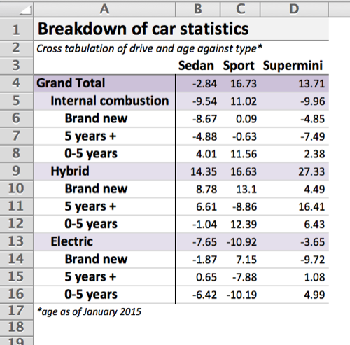
Excel Export with xltabr
Write crosstabs into Excel
devtools::install_github("moj-analytical-services/xltabr")
library(xltabr)

titles = c("Breakdown of car statistics", "Cross tabulation of drive and age against type*")
footers = "*age as of January 2015"
wb <- xltabr::auto_crosstab_to_wb(ct, titles = titles, footers = footers)
openxlsx::openXL(wb)
Given a crosstabulation ct produced by reshape2:dcast, the following table is generated.