5.2 Functions
Function arguments fall into two sets:
- data argument: give input data to compute on
- detail argument: control details of the computation
You can refer to an argument by its unique prefix. That is, partial matching is acceptable. But this is generally best avoided to reduce confusion.
When calling a function you can specify arguments by position, by complete name, or by partial name. Arguments are matched
- first by exact name (perfect matching),
- then by prefix matching, and
- finally by position.
If you specify arguments by names (full or partial), you can specify them in any order. If you specify arguments by position, you must specify them in the order they are defined in the function.
Example:
Here is a read.csv() function.
read.csv(file, header = TRUE, sep = ",", quote = "\"",
         dec = ".", fill = TRUE, comment.char = "", ...)
If you call
it will read the file path/to/file.csv with default values for all other arguments.
But if you call
this will return an error because FALSE is assigned to file and the filename is assigned to the argument header.
You can run.
To summarize:
- You can pass the arguments to
read.csvwithout naming them if they are in the order thatRexpects. - However, the order of the arguments matter if they are not named.
When you call a function and specify arguments, it is recommended to put a space around =, also put a space after a comma, not before.
x <- 10; y <- 5
x + y
#> [1] 15
`+`(x, y)
#> [1] 15

# ----------------------------
for (i in 1:2) print(i)
#> [1] 1
#> [1] 2
`for`(i, 1:2, print(i))
#> [1] 1
#> [1] 2

# ----------------------------
x[3]
#> [1] NA
# Note that only need to call the open braket
`[`(x, 3)
#> [1] NA

# ----------------------------
{ print(1); print(2); print(3) }
#> [1] 1
#> [1] 2
#> [1] 3
`{`(print(1), print(2), print(3))
#> [1] 1
#> [1] 2
#> [1] 3

# ----------------------------
sapply(1:5, `+`, 3)
#> [1] 4 5 6 7 8
sapply(1:5, "+", 3)
#> [1] 4 5 6 7 8
Note the difference between + and "+". The first one is the value of the object called +, and the second is a string containing the character +. The second version works because sapply can be given the name of a function instead of the function itself: if you read the source of sapply(), you’ll see the first line uses match.fun() to find functions given their names.
Every operation is a function call
Every operation in R is a function call, whether or not it looks like one. This includes infix operators like +, control flow operators like for, if, and while, subsetting operators like [] and $, and even the curly brace {. This means that each pair of statements in the following example is exactly equivalent. Note that `, the backtick, lets you refer to functions or variables that have otherwise reserved or illegal names:
5.2.1 Inspecting Object Types and Structure
str(x), class(x), and typeof(x)
str(x) focus on the structure not the contents. The output of the str() will vary depending on the type of R object you are passing it.
- For a data frame, the output will show the names of the columns, the class of each column, and the first few rows of data.
- For a list, the output will show the names of the elements in the list, the class of each element, and the value of each element.
class(x) returns a class attribute, a character vector giving the names of the classes from which the object inherits. 变量的类型, eg., dataframe, tibble, vector.
- If the object does not have a class attribute, it has an implicit class, notably
"matrix","array","function"or"numeric"or the result oftypeof(x). - A property (属性) assigned to an object that determines how generic functions operate with it. It is not a mutually exclusive classification. If an object has no specific class assigned to it, such as a simple numeric vector, it’s class is usually the same as its mode, by convention.
library(tibble)
DT <- tibble(a = rnorm(1000), b = rnorm(1000))

DT %>% class()
[1] "tbl_df"     "tbl"        "data.frame"

DT %>% str()
tibble [1,000 × 2] (S3: tbl_df/tbl/data.frame)
 $ a: num [1:1000] 1.327 1.71 -0.414 0.515 -0.117 ...
$ b: num [1:1000] -0.778 1.508 0.816 0.5 -1.874 ...str()is more informative thanclass().str()includes the class information, but also provides additional details about the structure of the object, such as the number of rows and columns (for data frames), the types of each column, and a preview of the data contained within the object.
typeof determines the (R internal) type or storage mode of any object. 变量里面存储数据的类型, eg., string, numeric, integer.
- Current values are the vector types
"logical","integer","double","complex","character","raw"and"list","NULL","closure"(function),"special"and"builtin"(basic functions and operators),"environment","S4"(some S4 objects) and others that are unlikely to be seen at user level ("symbol","pairlist","promise","language","char","...","any","expression","externalptr","bytecode"and"weakref"). mode(x)is similar totypeof(x)- mutually exclusive. One object has one
typeofandmode.
methods(class="zoo") get a list of functions that have zoo-methods.
attributes(x) returns the object’s attributes/metadata as a list. Some of the most common attributes are: row names and column names, dimensions, and class.
- Attributes are not stored internally as a list and should be thought of as a set and not a vector, i.e, the order of the elements of
attributes()does not matter. - To access a specific attribute, you can use the
attr()function.
attr(x, which) Get or set specific attributes of an object.
xan object whose attributes are to be accessed.whicha character string specifying which attribute is to be accessed.
attr(x, which) <- value specify value to the attribute
valuean object, the new value of the attribute, orNULLto remove the attribute.
# create a 2 by 5 matrix
> x <- 1:10
> attr(x, "dim") <- c(2, 5)
> x
     [,1] [,2] [,3] [,4] [,5]
[1,]    1    3    5    7    9
[2,]    2    4    6    8   10

> my_factor <- factor(c("A", "A", "B"), ordered = T, levels = c("A", "B"))
> my_factor
[1] A A B
Levels: A < B

> attributes(my_factor)
$levels
[1] "A" "B"

$class
[1] "ordered" "factor"
Q: What does 1L mean?
A: 1L is a shorthand for as.integer(1). Adding suffix L ensures that the value is treated as an integer and it is useful for memory usage and specific computations involving integer operations.
# create numerical value
num_val <- 1

# check the data type
print(class(num_val))
[1] "numeric"

print(typeof(num_val))
[1] "double"
# create integer value
int_val <- 1L
# check the data type
print(class(int_val))
[1] "integer"
print(typeof(int_val))
[1] "integer"5.2.2 Type of Variables
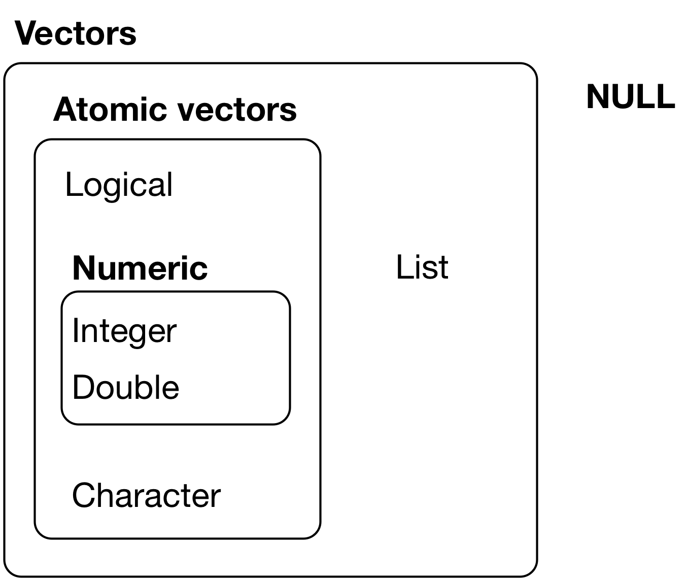
There are two types of vectors:
- Atomic vectors, of which there are six types: logical, integer, double, character, complex, and raw. Integer and double vectors are collectively known as numericvectors.
- Lists, which are sometimes called recursive vectors because lists can contain other lists.
The chief difference between atomic vectors and lists is that atomic vectors are homogeneous, while lists can be heterogeneous. There’s one other related object: NULL. NULL is often used to represent the absence of a vector (as opposed to NAwhich is used to represent the absence of a value in a vector). NULL typically behaves like a vector of length 0. The Figure below summarises the interrelationships.
Dimension Reduction
Convert a data frame, tibble, list to an atomic vector
unlist(df) or as.matrix(df) %>% as.vector()
Convert a matrix to a vector
as.vector(x)
unlist() TL;DR: takes in a list, returns a vector.
It “un-lists” nested lists or vectors and converts them into a simple atomic vector. In other words, it takes a list that contains other lists, vectors, or atomic elements and flattens it into a single vector.
- Useful when flatten a nested or hierarchical list to a vector. Dimension reduction.
- Simplifying the structure of a data object
- Passing a list to a function that only accepts vectors
- Combining the elements of a list into a single vector
> list(1, 2, 3, 4, 5)
  [[1]]
  [1] 1

  [[2]]
  [1] 2

  [[3]]
  [1] 3

    [[4]]
    [1] 4

    [[5]]
    [1] 5

> list(1, 2, 3, 4, 5) %>% unlist()
    [1] 1 2 3 4 5
# flatten a nested list
> list(a = 1, b = list(c = 2, d = 3), e = 4) %>% unlist()
  a b.c b.d   e
  1   2   3   4
> data.frame(matrix(1:12,3,4)) %>% unlist() # flatten by column
X11 X12 X13 X21 X22 X23 X31 X32 X33 X41 X42 X43
  1   2   3   4   5   6   7   8   9  10  11  12
5.2.3 Variable Scope
with(data, expr, …) Evaluate an R expression, expr, in an environment constructed from data, possibly modifying (a copy of) the original data.
expra single expression or a compounded one, i.e., of the form
within(data, expr, …) is similar to with, except that it examines the environment after the evaluation of expr and makes the corresponding modifications to a copy of data (this may fail in the data frame case if objects are created which cannot be stored in a data frame), and returns it.
- Returned value:
- For
within, the modified object. - For
with, the value of the evaluatedexpr.
- For
with(mtcars, mpg[cyl == 8  &  disp > 350])
# is the same as, but nicer than
mtcars$mpg[mtcars$cyl == 8  &  mtcars$disp > 350]
5.2.4 Control Structures
Note all keywords are lowercase here.
A ‘do … until’ loop in R:
repeat {
  # code
  if(stop_condition_is_true) break
}

while(TRUE){
  # Do things
  if (stop_condition_is_true) break
}
break statement can break out of a loop.
next statement causes the loop to skip the current iteration and start the next one.
switch(exp, case1, case2, ...) the expression is matched with the list of values and the corresponding value is returned.
a <- 4
switch(a,
       "1"="this is the first case in switch",
       "2"="this is the second case in switch",
       "3"="this is the third case in switch",
       "4"="this is the fourth case in switch",
       "5"="this is the fifth case in switch"
       )
ifelse(test_expression, x, y)
The returned vector has element from x if the corresponding value of test_expression is TRUE; or from y if the corresponding value of test_expression is FALSE.
That is the i-th element of result will be x[i] if test_expression[i] is TRUE else it will take the value of y[i].
ref: