3.10 Render Jupyter notebook

You can use quarto to convert Jupyter notebooks (.ipynb) to other formats such as HTML, PDF, or Markdown. It uses the document YAML to decide which format to convert to.

quarto render notebook.ipynb

Note that when rendering an .ipynb Quarto will NOT execute the cells within the notebook by default (the presumption being that you already executed them while editing the notebook). If you want to execute the cells you can pass the --execute flag to render:

quarto render notebook.ipynb --execute

Path error when rendering .ipynb file with quarto --execute:

quarto render 07_Lab-2_dummy-variable.ipynb --execute --log-level=DEBUG
Quarto version: 1.7.31
projectContext: Found Quarto project in /Users/menghan/Library/CloudStorage/OneDrive-Norduniversitet/FIN5005 2025Fall/course_web
Loaded deno-dom-native
[execProcess] python /Applications/quarto/share/capabilities/jupyter.py
[execProcess] Success: true, code: 0

Starting ir kernel...[execProcess] /Users/menghan/anaconda3/bin/python /Applications/quarto/share/jupyter/jupyter.py
[execProcess] Success: true, code: 0
ERROR: 

path
[NotebookContext]: Starting Cleanup

Not resolved…

---

3.10.1 Code cell modes

Three code modes in Jupyter notebooks:

• Unselected: When no bar is visible, the cell is unselected.

• Selected: When a cell is selected, it can be in command mode or in edit mode.

  • Command mode: solid vertical bar on the left side of the cell. 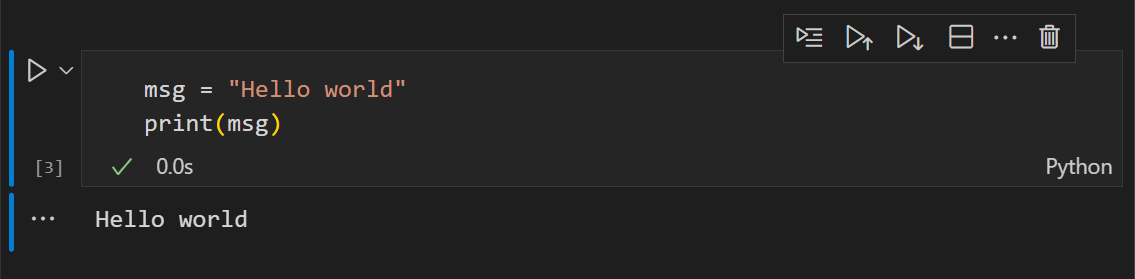The cell can be operated on and accepts keyboard commands.

    Hit Enter to enter edit mode, or click on the cell to enter edit mode.

  • Edit mode: a solid vertical bar is joined by a blue border around the cell input editor. Press Escape to return to command mode, or click outside the cell to return to command mode.

---

3.10.2 Keyboard shortcuts

Command Palette, type “Preferences: Open Keyboard Shortcuts” to open the keyboard shortcuts editor. You can search for “jupyter” to find all Jupyter-related commands and their shortcuts.

Run code cells

Shortcut	Function
Ctrl+Enter	runs the currently selected cell; focus stays on the current cell
Shift+Enter	runs the currently selected cell and focus moves to new cell.
Opt+Enter	runs the currently selected cell and inserts a new cell immediately below (focus moves to new cell).
Run Cells Above	Command Palette, type “Notebook: Execute Above Cells”

There is no executing current cell and moving focus to the next cell shortcut, you need to first run the current cell with Ctrl+Enter, then hit the down arrow key ↓ to move focus to the next cell.

I added one keyboard shortcut for this: cmd+Enter to run the current cell and move focus to the next cell. This works for both command mode and edit mode.

{
  "key": "cmd+enter",
  "command": "notebook.cell.executeAndSelectBelow",
  "when": "notebookEditorFocused"
}

Insert code cells

Under command mode (no thin blue border around the input cell, one thick vertical bar on the left):

Shortcut	Function
ctrl+; A	Press Ctrl+;, release, then A. Insert a new code cell above the current one.
ctrl+; B	Add a new code cell below the selected one.

Note: On my Mac, I just need to hit ESC to enter command mode, then A or B to insert a new cell above or below the current cell. No need to hit Ctrl+; first.

Change Cell to Code

Shortcut	Function
cmd mode: Y	Change cell to code
cmd mode: M	Change cell to Markdown

Miscellaneous

Shortcut	Function
ctrl+; X or dd	Delete selected cells
shift + ↑/↓	Select consecutive multiple cells
L	command mode; toggle line numbers
R	Undo last change

ref:

• Most useful keyboard shortcuts for Notebook & Lab
• Jupyter Tutorial

3.10.3 Insert Image

The built-in image rendering in Jupyter notebooks is not very flexible. It renders images using the default width and height (about 50% of page width and almost square), which might be too large or too small for your needs, and very often, you want a specific aspect ratio.

Use IRdisplay to control plot size in Jupyter notebooks: ✅

1. generate the image and save it to a file, e.g., temp-plot.png

   ggsave(f_name, p, width = 6, height = 4, dpi = 300, units = "in")

2. insert a code cell and load the image using IRdisplay::display_html()

   #| echo: false
   # Display the image with controlled width using HTML
   library(IRdisplay)
   display_html(paste0('<img src="', f_name, '" style="width: 70%; height: auto;">'))
   # center the image
   display_html(paste0('<div style="text-align: center;"><img src="', f_name, '" style="width: 70%; height: auto;"></div>'))

Alternatively, use markdown syntax

![Alt text](temp-plot.png){width=70%}

• Plot size with IRKernel

---

repr options

repr options are used to control the behavior of repr when not calling it directly. Use options(repr.* = ...)and getOption('repr.*') to set and get them, respectively.

Once repr package is loaded, all options are set to defaults which weren’t set beforehand.

repr.plot.*: representations of recordedplot instances

Options	Descriptions
repr.plot.width	Plotting area width in inches (default: 7 in)
repr.plot.height	Plotting area height in inches (default: 7 in)
repr.plot.pointsize	Text height in pt (default: 12)
repr.plot.res	PPI for rasterization (default: 120)

# set plot size to 4 x 3 inches
options(repr.plot.width = 4, repr.plot.height = 3)

This works but is not ideal as the plot element is not adjusted proportionally. Text size is too large for the small plot and might be cropped. ❌

Other output representations

Options	Descriptions
repr.matrix.max.rows	How many rows to display at max. Will insert a row with vertical ellipses to show elision. (default: 60 rows, first and last 30 rows)
repr.matrix.max.cols	How many cols to display at max. Will insert a column with horizontal ellipses to show elision. (default: 20)

See repr CRAN for all available options.

---

3.10.4 View data frames

Jupyter Notebook comes with a built-in Data Viewer. Choose ‘Jupyter Variables’ in the menu bar on the top, if you don’t see it, click the ‘…’ button to find it. It will show you all the variables in the terminal panel.

Tou can double-click a variable to open it in the Data Viewer. It provides a spreadsheet-like interface to view the data.

You can filter, sort, and search the data in the Data Viewer.

---

Data Wrangler

Use Data Wrangler extension to view data frames in a spreadsheet-like interface.

Launch Data Wrangler from a Jupyter Notebook

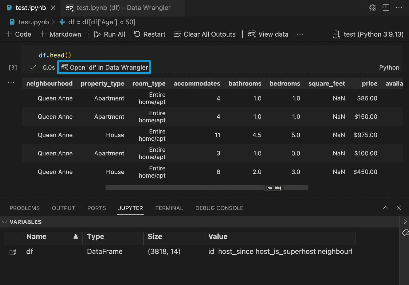
If you have a Pandas data frame in your notebook, you’ll now see an Open ‘df’ in Data Wrangler button (where df is the variable name of your data frame) appear in bottom of the cell after running any of df.head(), df.tail(), display(df), print(df), and df.

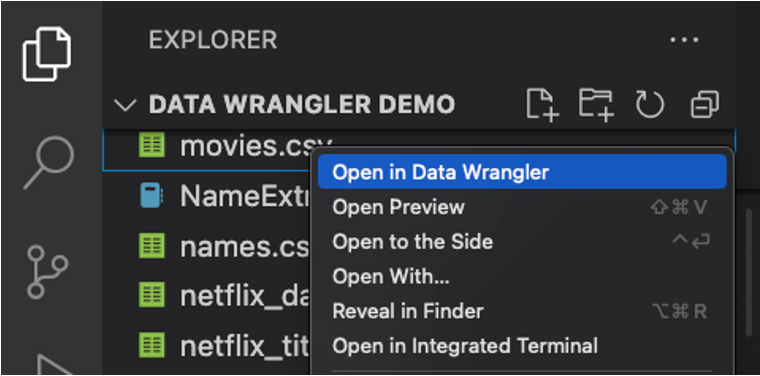
You can also launch Data Wrangler directly from a local file (such as a .csv). Right-click the file in the File Explorer and select Open in Data Wrangler.

ref: Quick Start Guide for Data Wrangler in VS Code

---

3.10.5 Export Jupyter notebook

You can export Jupyter notebooks to various formats, including Python scripts (.py), HTML, PDF, and more.

Refer to this post

The exported .py file will have “Run Cell”, “Run Below”, etc. This is due to # %% cell markers in the exported .py file. But they don’t interfere with the execution of the code in the .py file. Besides, I actually like these segmentation as they organize the code into sections and make it easier to run code in chunks. These features are useful when you run the .py file in an interactive window.

The trick part is you need to deal with the magic commands manually. .py files don’t support magic commands, so you need to remove them or replace them with equivalent python code.

---