11.5 Portfolio Return
PerformanceAnalytics is useful for portfolio analysis and performance analytics. It has functions to calculate portfolio return, risk, and performance metrics. Also good at visualizing portfolio performance and risk.
From asset parameters to portfolio parameters
Given a expected return and volatility for each asset, we can calculate the expected return and volatility of a portfolio by the following formulas:
\[ \begin{aligned} E[r_{p,t}] &= \sum_{i=1}^k w_{i,t} E[r_{i,t}] \\ \text{Var}[r_{p,t}] &= \sum_{i=1}^k\sum_{j=1}^k w_{i,t}\,w_{j,t}\,\text{Cov}(r_{i,t}, r_{j,t}) \end{aligned} \]
Given the following set up for two assets A and B:
| Asset A | Asset B | |
| \(\mu\) | 0.175 | 0.055 |
| \(\sigma\) | 0.258 | 0.115 |
| \(\rho_{AB}\) | -0.164 | |
where \(\mu\) is the expected return, \(\sigma\) is the volatility (standard deviation) of returns, \(\rho\) is the correlation coefficient between assets A and B.
Equally weighted
First we consider an equally weighted portfolio \(p_1\).
Asset weights: \(w_A = w_B = 0.5\).
ptf_par <- function(x.A, x.B, mu.A, mu.B, sig.A, sig.B, rho.AB) {
  # Calculate portfolio parameters given asset parameters and weights
  mu.p = x.A*mu.A + x.B*mu.B
  sig2.p = x.A^2 * sig.A^2 + x.B^2 * sig.B^2 + 2*x.A*x.B*rho.AB*sig.A*sig.B
  sig.p = sqrt(sig2.p)
  data.tbl = t(c(mu.p=mu.p, sig.p=sig.p, sig.avg=x.A*sig.A+x.B*sig.B))
  return(data.tbl)
}

# equally weighted portfolio
ptf_par(x.A=0.5, x.B=0.5, mu.A, mu.B, sig.A, sig.B, rho.AB)
## mu.p sig.p sig.avg
## [1,] 0.115 0.1323416 0.1865Long-short portfolio
We now consider a long-short portfolio \(p_2\).
Asset weights: \(w_A = 1.5\), \(w_B = -0.5\).
##       mu.p     sig.p sig.avg
## [1,] 0.235 0.4004673  0.3295
From individual asset returns to portfolio
Given a data frame of asset returns, we can calculate the portfolio return by PerformanceAnalytics::Return.portfolio().
w <- c(0.25, 0.25, 0.20, 0.20, 0.10)

portfolio_returns_xts_rebalanced_monthly <-
  Return.portfolio(asset_returns_xts, weights = w, rebalance_on = "months") %>%
  `colnames<-`("returns")
PerformanceAnalytics::Return.portfolio(R=Return_xts, weights=NULL, rebalance_on, verbose=FALSE) Using a time series of returns and any regular or irregular time series of weights for each asset, this function calculates the returns of a portfolio with the same periodicity of the returns data. Returns a time series of returns weighted by the weights parameter, or a list that includes intermediate calculations
RAn xts, vector, matrix, data frame, timeSeries or zoo object of asset returns.weightsA time series or single-row matrix/vector containing asset weights, as decimal percentages, treated as beginning of period (BOP) weights.If the user does not specify weights, an equal weight portfolio is assumed.
if
weightsis anxtsobject, then any value passed torebalance_onis ignored.This is useful when you have varying assets across time.
The
weightsindex specifies the rebalancing dates, therefore a regular rebalancing frequency provided viarebalance_onis not needed and ignored.Note that
weightsandRshould be matched by period.Irregular rebalancing can be done by specifying a time series of weights. The function uses the date index of the weights for xts-style subsetting of rebalancing periods.
rebalance_onDefault “none”; alternatively “daily” “weekly” “monthly” “annual” to specify calendar-period rebalancing supported byendpoints.- Ignored if
weightsis an xts object that specifies the rebalancing dates.
- Ignored if
verboaseIf verbose is TRUE, return a list of intermediary calculations, such as asset contribution and asset value through time.- The resultant list contains
$returns,$contributions,$BOP.Weight,$EOP.Weight,$BOP.Value, and$EOP.Value.
- The resultant list contains
chartSeries plot an OHLC object.
chartSeries(AMZN, type="candlesticks", subset='2016-05-18::2017-01-30', theme = chartTheme('white', up.col='green', dn.col='red'))type="candlesticks"can beline,bar, default tocandlesticks.A candle has four points of data:
- Open – the first trade during the period specified by the candle
- High – the highest traded price
- Low – the lowest traded price
- Close – the last trade during the period specified by the candle
A candle has three parts: body (open/close prices), upper shadow (high price), and lower shadow (low price).
The color of the body can tell them if the stock price is rising or falling. Usually, red stands for falling and green stands for rising.
theme = chartTheme("black")defaults to black theme.up.colup bar/candle colordn.coldown bar/candle color
11.5.1 Plot portfolio return
Use PerformanceAnalytics::charts.PerformanceSummary to plot the cumulative return, monthly return, and drawdown of a portfolio.
library(PerformanceAnalytics)
library(xts)

plot_png_base <- function(expr, f_name, width, height, ppi = 300,
                          trim = TRUE, pad = 8) {
  # For base-graphics plots (PerformanceAnalytics, plot.xts, ...), which draw
  # as a side effect rather than returning an object to print.
  #
  # trim = TRUE crops the blank border the device leaves around the plot.
  # charts.PerformanceSummary in particular reserves room for a title it is
  # not drawing, so a 9x7 canvas comes back 13% blank at the top -- which on a
  # slide reads as an unexplained gap between the figure and the text above.
  png(f_name, width = width * ppi, height = height * ppi, res = ppi)
  on.exit({
    invisible(dev.off())
    if (trim) trim_png(f_name, pad = pad)
  }, add = TRUE)
  force(expr) # the promise evaluates here, with the device open
  invisible(NULL)
}

trim_png <- function(f_name, pad = 8) {
  # Crop the uniform border off a png, then give it back `pad` pixels so the
  # ink does not touch the edge. Silently a no-op if magick is unavailable.
  if (!requireNamespace("magick", quietly = TRUE)) return(invisible(FALSE))
  img <- magick::image_read(f_name)
  img <- magick::image_trim(img)
  img <- magick::image_border(img, color = "white",
                              geometry = paste0(pad, "x", pad))
  magick::image_write(img, f_name)
  invisible(TRUE)
}

ret <- read.csv("data/etf_ARKK_case_study_monthly.csv")
ret$Date <- as.Date(ret$Date)

# Convert to xts
# col1: ptf return, col2: benchmark return
ret_xts <- xts(ret[, c("ptf_ret", "bmk_ret")], order.by = ret$Date)
colnames(ret_xts) <- c("ARK Innovation", "S&P 500")
# Risk-free rate for risk-adjusted performance measures
rf_xts <- xts(ret$rf, order.by = ret$Date)
colnames(rf_xts) <- "rf"

f_name <- "images/etf_ret_summary.png"
plot_png_base(
  charts.PerformanceSummary(ret_xts,
    main = "", legend.loc = "topleft",
    colorset = c("#b2182b", "#43418A")
  ),
  f_name, 9, 7
)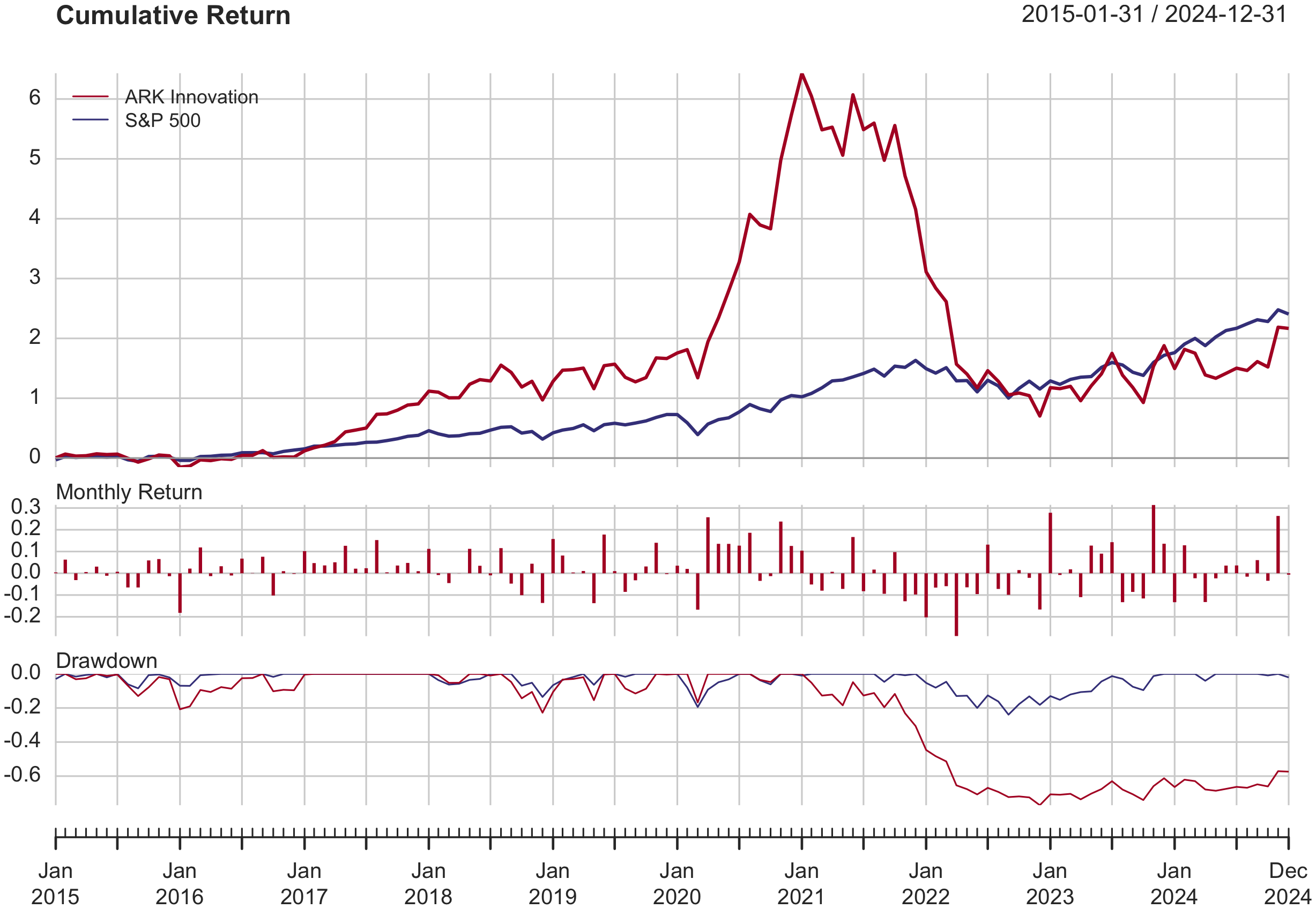
legend.loc: legend location, without it, the legend won’t show.There are nine locations that can be specified by keyword: “bottomright”, “bottom”, “bottomleft”, “left”, “topleft”, “top”, “topright”, “right” and “center”.
colorset: color palette to use. You can specify a vector of colors, or use one of the built-in color palettes.Legend is ordered by the order of the columns.
colorset = c("#b2182b", "#43418A")will set the first series to#b2182band the second series to#43418A.
Drawdown analysis: https://metricgate.com/docs/drawdown-analysis/
Drawdown: It is the level of losses from the last value of peak equity attained. \[ D_t = \frac{V_t-\text{max}_{s<t}V_s}{\text{max}_{s<t}V_s} \] where \(V_t=\Pi_{s=1}^t(1+R_S)\) is the cumulative portfolio value at time \(t\) and \(\text{max}_{s<t}V_s\) is the maximum cumulative portfolio value attained prior to time \(t\).
Since drawdown represents a loss, \(D_t\le 0\) always.
Maximum Drawdown: minimum value of the drawdown over a specified time period. \[ \text{Max Drawdown} = \min_t(D_t) \]
##         From     Trough         To   Depth Length To Trough Recovery
## 1 2021-02-28 2022-12-31       <NA> -0.7708     48        23       NA
## 2 2018-09-30 2018-12-31 2019-07-31 -0.2277     11         4        7
## 3 2015-06-30 2016-01-31 2016-09-30 -0.2075     16         8        8
## 4 2020-03-31 2020-03-31 2020-04-30 -0.1673      2         1        1
## 5 2019-08-31 2019-09-30 2019-11-30 -0.1149      4         2        2
Trough: The lowest point reached during a drawdown episode before recovery begins.
Drawdown Duration: The full length of a drawdown episode from peak to the next new peak, encompassing both the decline and recovery phases.
High-Water Mark: The highest cumulative value ever achieved; drawdown is always measured relative to this level.
The drawdown at any particular time point is simply the distance from the current variable value to the “surface of the water” or the high water mark at that time point.
Plot the high-water mark together with the wealth index:
wealth <- cumprod(1 + ret_xts[, 1]) # wealth index, $1 invested at the start
hwm <- cummax(wealth) # high-water mark, the running max of the wealth index
dd <- wealth / hwm - 1 # drawdown, identical to Drawdowns(ret_xts[, 1])

wi <- merge(wealth, hwm)
colnames(wi) <- c("Wealth index", "High-water mark")
band <- merge(hwm, wealth) # upper bound first, lower bound second

f_name <- "images/etf_hwm.png"
plot_png_base({
  p <- plot(wi,
    col = c("black", "blue"), lwd = c(2, 1.5),
    main = "", legend.loc = "topleft"
  )
  # shade the underwater area, i.e. the gap between the two lines
  p <- addPolygon(band, col = adjustcolor("blue", alpha.f = 0.15), on = 1)
  print(p)
}, f_name, 11, 6, trim = FALSE)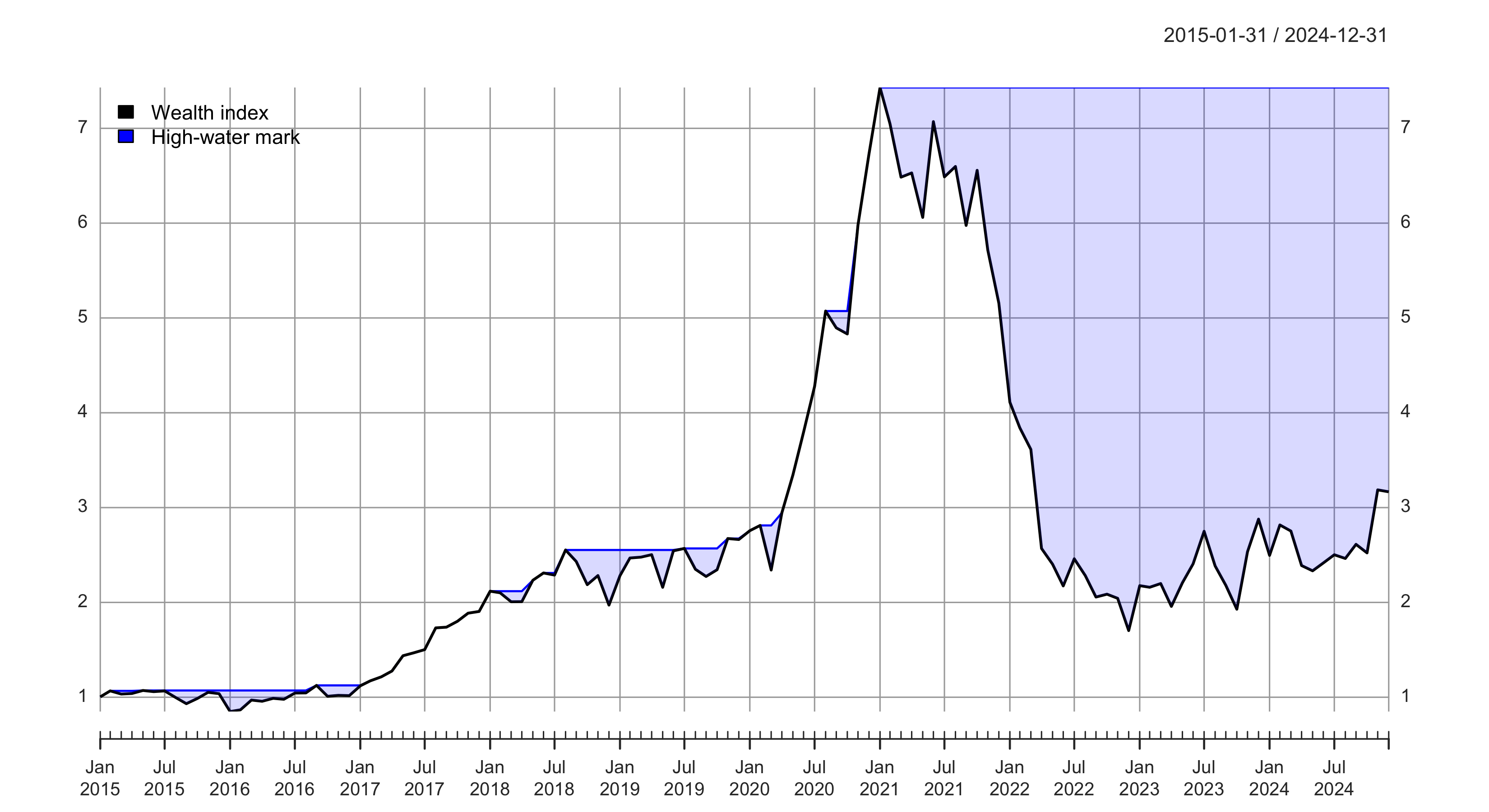
cumprodandcummaxare applied column by column on anxtsobject, so the same two lines work on all columns ofret_xtsat once.Rename the columns of the merged object, otherwise both series are labelled
ARK.Innovationin the legend.addPolygonfills the area between the first two columns of the object it is given, the first being the upper bound and the second the lower bound.on = 1draws it on the existing panel; without it the polygon goes into a new panel below.Use a transparent fill (
adjustcolor(col, alpha.f = 0.15)), since layers are drawn in the order they are added and the polygon lands on top of the two lines.addPolygonandaddSeriesreturn the plot object instead of drawing it, so it has to beprinted. Inside a knitr chunk this is needed forplotas well, since auto-printing does not happen there.To add the drawdown as a separate panel below, add
p <- addSeries(dd, col = "#43418A", type = "h", lwd = 2, main = "Drawdown from high-water mark")beforeprint(p).
11.5.2 Rolling performance
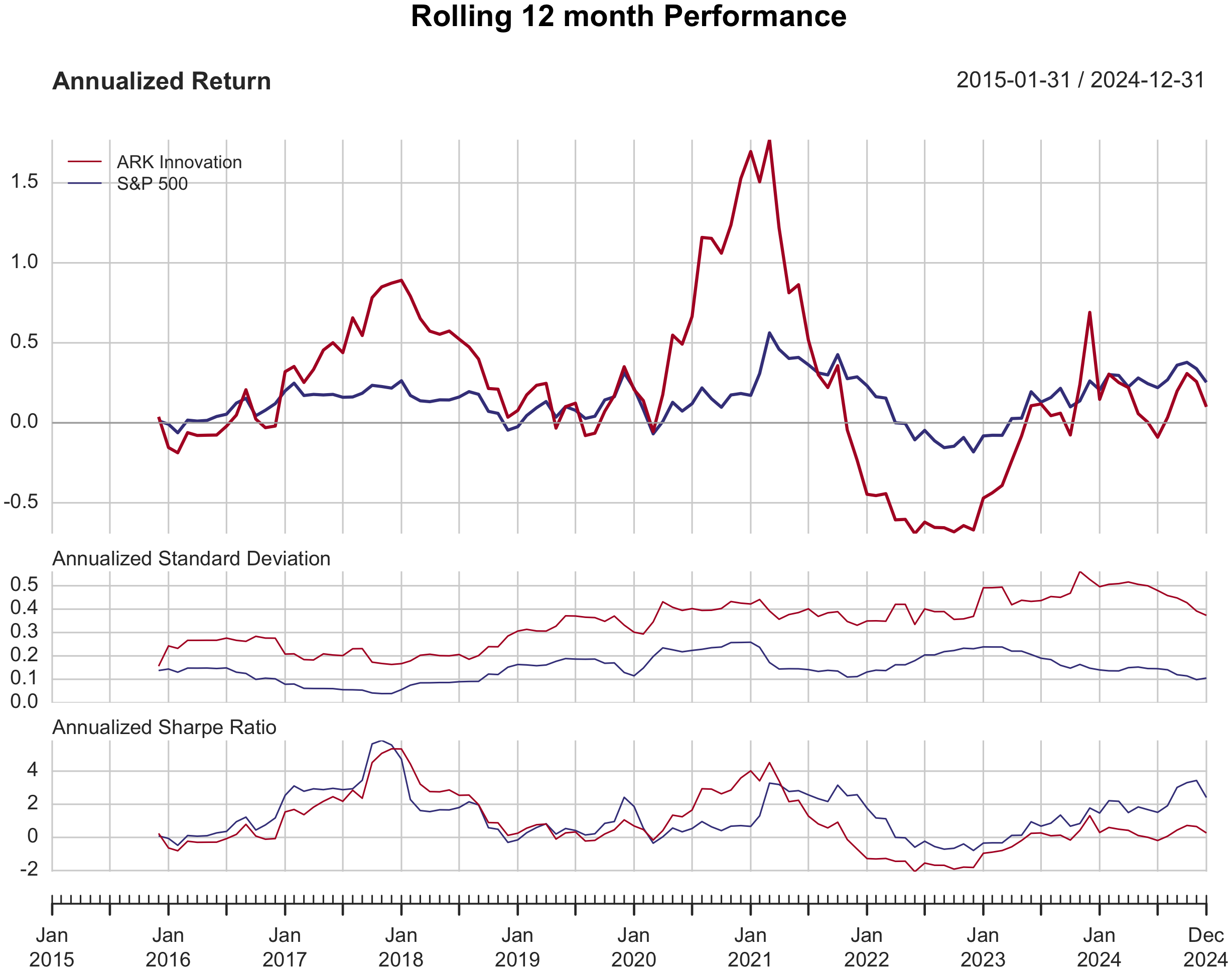
charts.RollingPerformance(R, width=12) creates a rolling annualized returns chart, rolling annualized standard deviation chart, and a rolling annualized sharpe ratio chart.
Note that if your portfolio return is on a daily basis, first convert to monthly, then run the rolling function. Otherwise, daily rolling frequency can be too computationally intensive.
Rolling window
Rolling window estimation
Example:
f_name <- "images/etf_ret_rolling.png"
plot_png_base(
  charts.RollingPerformance(
    R = ret_xts, Rf = rf_xts$rf, width = 12,
    legend.loc = "topleft", colorset = c("#b2182b", "#43418A")
  ),
  f_name, 9, 7
)
11.5.3 Monthly summary statistics
Use PerformanceAnalytics::table.Stats() to calculate summary statistics for a portfolio.
| ARK Innovation | S&P 500 | |
|---|---|---|
| Observations | 120.0000 | 120.0000 |
| NAs | 0.0000 | 0.0000 |
| Minimum | -0.2890 | -0.1249 |
| Quartile 1 | -0.0535 | -0.0164 |
| Median | 0.0083 | 0.0165 |
| Arithmetic Mean | 0.0150 | 0.0112 |
| Geometric Mean | 0.0097 | 0.0103 |
| Quartile 3 | 0.0774 | 0.0370 |
| Maximum | 0.3144 | 0.1270 |
| SE Mean | 0.0095 | 0.0040 |
| LCL Mean (0.95) | -0.0039 | 0.0032 |
| UCL Mean (0.95) | 0.0339 | 0.0192 |
| Variance | 0.0109 | 0.0020 |
| Stdev | 0.1045 | 0.0442 |
| Skewness | 0.2209 | -0.3871 |
| Kurtosis | 0.4032 | 0.4356 |
SE Mean: Standard Error of the average return. \[\text{SE Mean} = \frac{\sigma_p}{\sqrt{T}}\]LCL Mean: Lower Confidence Level (LCL) of the mean, defaults to 95% confidence level. \[\text{LCL Mean} = \bar{r}_p - \text{SE Mean} \times c_{\alpha/2}\] where \(c_{\alpha/2}\) is the critical value, i.e., \(\left(1-\frac{\alpha}{2}\right)\) quantile of the \(t\) distribution with \((T-1)\) degrees of freedom.UCL Mean: Upper Confidence Level (UCL) of the mean, defaults to 95% confidence level. \[\text{UCL Mean} = \bar{r}_p + \text{SE Mean} \times c_{\alpha/2}\]Kurtosis: Excess Kurtosis.
Downside risk measures
Semi-deviation, Value at Risk (VaR), and Expected Shortfall (ES) are downside risk measures that focus on the negative returns of a portfolio.
# Downside risk measures
library(tidyverse)
stats <- table.Stats(ret_xts, digits = 4)
rbind(
  stats["Stdev", ],
  SemiDeviation(ret_xts),
  VaR(ret_xts, p = 0.05),
  ES(ret_xts, p = 0.05)
) %>%
  kable(digit = 4) %>%
kable_styling(full_width = FALSE)| ARK Innovation | S&P 500 | |
|---|---|---|
| Stdev | 0.1045 | 0.0442 |
| Semi-Deviation | 0.0710 | 0.0330 |
| VaR | -0.1487 | -0.0655 |
| ES | -0.1897 | -0.0910 |
Standard deviation measures total risk; semi-deviation only the downside volatility.
\(\text{VaR(5%)}_{\text{ARK}}=15.87\%\): There is a 5% chance that ARK loses more than \(14.87\%\) over one month. Or, equivalently, there is a 95% chance that ARK loses less than \(14.87\%\) over one month. The index’s VaR is \(6.55\%\).
\(\text{ES(5%)}_{\text{ARK}}=18.97\%\): given that ARK is in the worst 5% of months, it will lose on average \(18.97\%\). The index’s ES is \(9.95\%\).
11.5.4 Risk-adjusted performance measures
Sharpe ratio
sharpe <- SharpeRatio(ret_xts, Rf = rf_xts, geometric = FALSE)
sharpe %>%
  kable(digits = 4) %>%
kable_styling(full_width = FALSE)| ARK Innovation | S&P 500 | |
|---|---|---|
| StdDev Sharpe (Rf=0.1%, p=95%): | 0.1301 | 0.2226 |
| VaR Sharpe (Rf=0.1%, p=95%): | 0.0914 | 0.1502 |
| ES Sharpe (Rf=0.1%, p=95%): | 0.0716 | 0.1082 |
| SemiSD Sharpe (Rf=0.1%, p=95%): | 0.1352 | 0.2110 |
Annualized Sharpe ratio
sharpe_ann <- SharpeRatio.annualized(ret_xts, Rf = rf_xts, geometric = FALSE)
sharpe_ann %>%
  kable(digits = 4) %>%
kable_styling(full_width = FALSE)| ARK Innovation | S&P 500 | |
|---|---|---|
| Annualized Sharpe Ratio (Rf=1.7%) | 0.4506 | 0.771 |
CAPM-related performance measures
Calculate Beta, Alpha, R-squared, Information ratio, Treynor ratio of a portfolio against a benchmark.
table.CAPM(Ra, Rb, scale = NA, Rf = 0, digits = 4) or table.SFM will show statistics pertaining to an asset against a set of benchmarks, or statistics for a set of assets against a benchmark.
Ra: a vector of asset returns to be examinedRb: a matrix of benchmark returns to test the asset againstRf: risk-free rate of return, defaults to 0scale: number of periods in a year (daily scale = 252, monthly scale = 12, quarterly scale = 4)digits: number of decimal places to round to,
capm <- table.CAPM(
  Ra = ret_xts[, 1], Rb = ret_xts[, 2],
  Rf = rf_xts$rf, scale = 12, digits = 4
)
capm %>%
  kable() %>%
kable_styling(full_width = FALSE)| ARK Innovation to S&P 500 | |
|---|---|
| Alpha | -0.0032 |
| Beta | 1.7053 |
| Alpha Robust | -0.0038 |
| Beta Robust | 1.6880 |
| Beta+ | 1.8379 |
| Beta- | 1.5617 |
| Beta+ Robust | 1.8070 |
| Beta- Robust | 1.6146 |
| R-squared | 0.5205 |
| R-squared Robust | 0.4704 |
| Annualized Alpha | -0.0377 |
| Correlation | 0.7215 |
| Correlation p-value | 0.0000 |
| Tracking Error | 0.2728 |
| Active Premium | -0.0082 |
| Information Ratio | -0.0301 |
| Treynor Ratio | 0.0608 |
Returned values
Beta: beta coefficient of CAPMBeta +:CAPM.beta.bullis a regression for only positive market returns, which can be used to understand the behavior of the asset or portfolio in positive or ‘bull’ markets.Beta -:CAPM.beta.bearprovides the calculation on negative market returns.Active Premium: performance premium provided by an investment over a passive strategy (the benchmark), which is the investment’s annualized return minus the benchmark’s annualized return. Also called “Active Return.” \[ \text{Active Premium} = \bar{r}_p-\bar{r}_m \]Tracking Error: the unexplained portion of the investment’s performance relative to a benchmark, defined as the standard deviation of the active return. \[ \begin{aligned} \text{Tracking Error} &= \sigma_{p-m} \\ &= \sqrt{\frac{\sum(r_{p}-r_{m})^{2}}{T-1}} \times \sqrt{\text{scale}} \end{aligned} \] \(\text{scale}\) is the number of periods in a year (daily scale = 252, weekly scale = 52, monthly scale = 12, quarterly scale = 4, annually sacle = 1).Information Ratiois defined as theActive Premiumdivided by theTracking Error. \[ \begin{aligned} \text{IR}_p &= \frac{\text{Active Premium}}{\text{Tracking Error}} \\ &= \frac{\bar{r}_p-\bar{r}_m}{\sigma_{p-m}} \end{aligned} \]
Risk decomposition of the return distribution.
Specific risk is the annualized standard deviation of the error term in the CAPM regression equation.
Systematic risk, as defined by Bacon (2008), is the product of beta by market risk. \[ \sigma_s = \beta * \sigma_m \] Market risk, \(\sigma_m\), is the annualized standard deviation of the benchmark. \(\beta\) is the regression beta.
Total risk is defined as \[ \text{Total Risk} = \sqrt{\text{Systematic Risk}^2 + \text{Specific Risk}^2} \]
# Risk decomposition
risk <- table.SpecificRisk(
  Ra = ret_xts[, 1], Rb = ret_xts[, 2],
  Rf = rf_xts$rf, digits = 4
)
risk %>%
  kable() %>%
kable_styling(full_width = FALSE)| ARK Innovation | |
|---|---|
| Specific Risk | 0.2495 |
| Systematic Risk | 0.2611 |
| Total Risk | 0.3630 |